13 Central Limit Theorem(중심 극한 정리)
13.1 히스토그램
- 구간을 만들고, 구간에 해당되는 값들의 개수를 카운트하여 막대로 표시한 그래프
- 분포(distribution)을 만들 때 좋다.
13.2 연구와 추론

13.3 중심극한정리
The Central Limit Theorem for sample means in statistics states that, given a sufficiently large sample size, the sampling distribution of the mean for a variable will approximate a normal distribution regardless of the variable’s underlying distribution of the population observations:
\[ \bar{X} \sim N(\mu, \frac{\sigma^2}{n}) \]
표본 평균에 대해서 중심극한 정리를 적용해 보았을 때,
어떤 모집단의 (확률)변수가 어떤 분포를 따르는지에 상관없이,
충분히 샘플이 크면,
샘플의 평균들의 분포(평균의 샘플링 분포)는 평균이 \(\mu\)이고, 분산이 \(\frac{\sigma^{2}}{n}\)인 정규분포를 따른다.
분산의 (양의) 제곱근이 표준편차이다. 이 분포의 표준편차 \(\sqrt{\frac{\sigma^{2}}{n}}\)를 SEM(Standard Error of the Mean)이라고도 한다.
평균 이외에도 다른 통계량(statistic)에도 적용할 수 있지만, 평균에 적용하는 경우가 가장 흔하다.
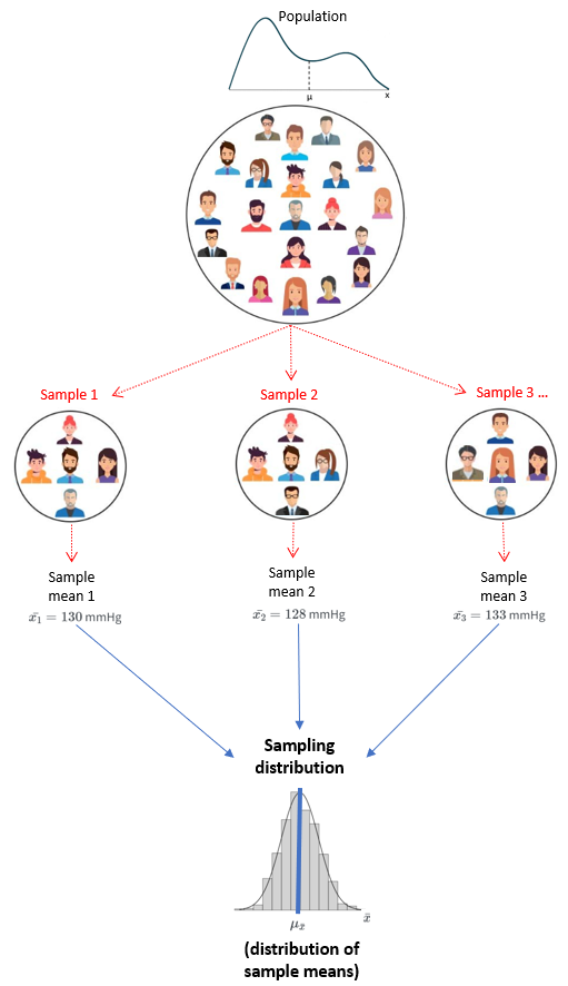
13.4 평균의 샘플링 분포(Sampling distribution of the mean)
13.5 R 코드 시뮬레이션
13.6 Confidence Interval(신뢰구간)

\[ 95\%CI = \mu_{\bar{x}} \pm 1.96 \, \sigma_{\bar{x}} = \mu_{\bar{x}} \pm 1.96 \, \frac{\sigma}{\sqrt{n}} \]
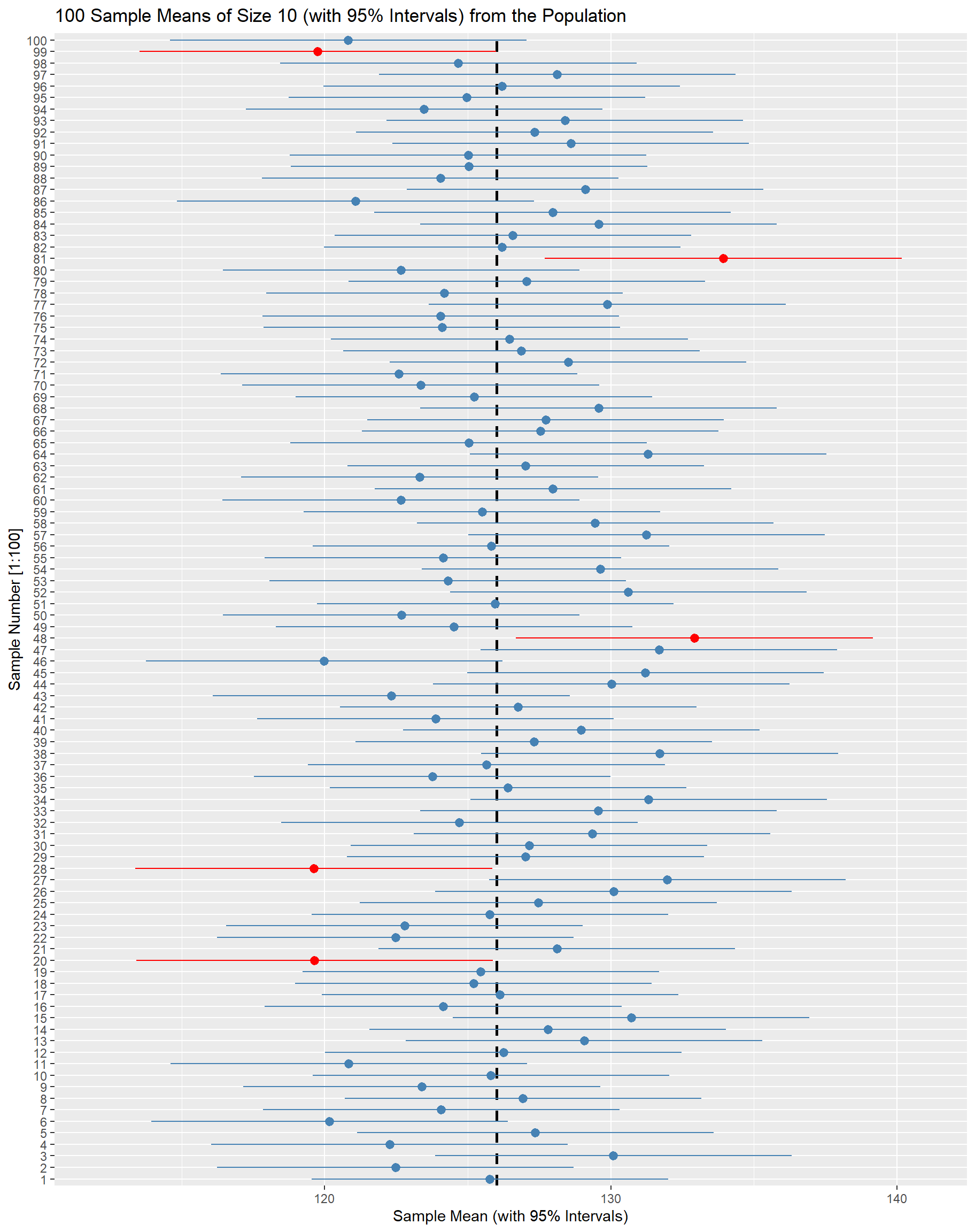
13.6.1 신뢰구간의 의미
- 아래 그림에서 인용된 책을 읽어 보자.

- (Sedgwick 2014)도 읽어 보자.