인터넷에는 이 데이터셋을 사용한 통계 분석 및 머신러닝 관련된 자료들도 많이 찾을 수 있다.
이 데이터셋은 워킹 디렉터리의 data 서브 디렉터리에 healthcare-dataset-stroke-data.csv라는 이름으로 저장되어 있다고 생각해 보자. 이 파일의 확장자는 .csv로 “Comma-Separated Values file”이다. 플레인 텍스트로 되어 있고, 코마로 값들을 구분한다. CSV 파일은 엑셀로도 쉽게 읽을 수 있고, 엑셀에서 쉽게 CSV로 저장할 수도 있으며, 플레인 텍스트이기 때문에 아무 텍스트 편집기로도 읽을 수 있어서 데이터 과학에서 자주 사용된다.
readr이라는 패키지의 read_csv() 함수를 사용하여 파일을 읽는다. 이 함수는 데이터를 tibble(R 데이터프레임을 보강한 것)로 가지고 온다. (아직 우리가 tibble을 배우지 않아서) 원래의 R 데이터프레임으로 바뀌기 위해서 as.data.frame()를 사용했다.
library(readr)stroke_df <-as.data.frame(read_csv("data/healthcare-dataset-stroke-data.csv"))head(stroke_df) # 앞 6개의 행
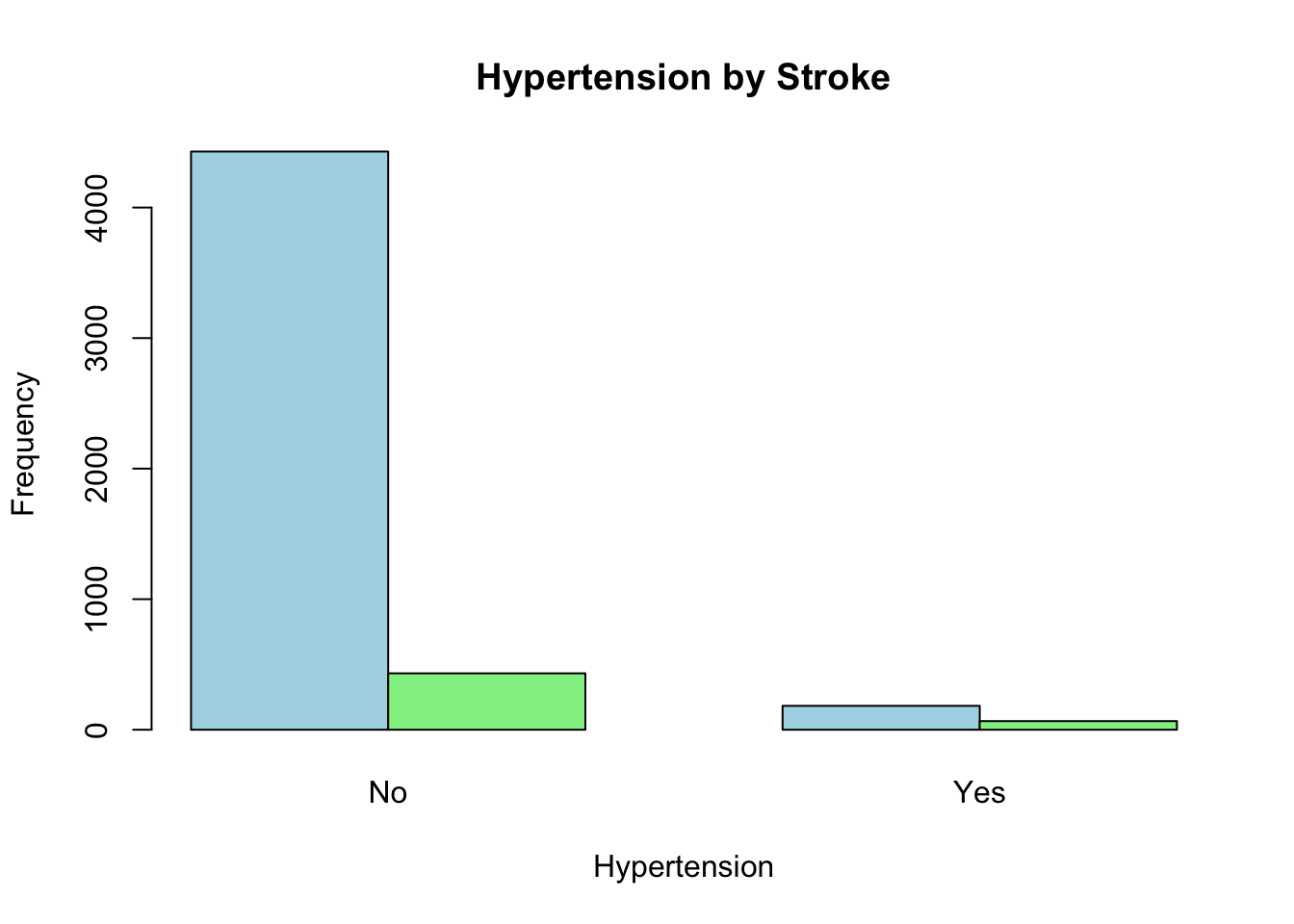
hypertension: 0 if the patient doesn’t have hypertension, 1 if the patient has hypertension
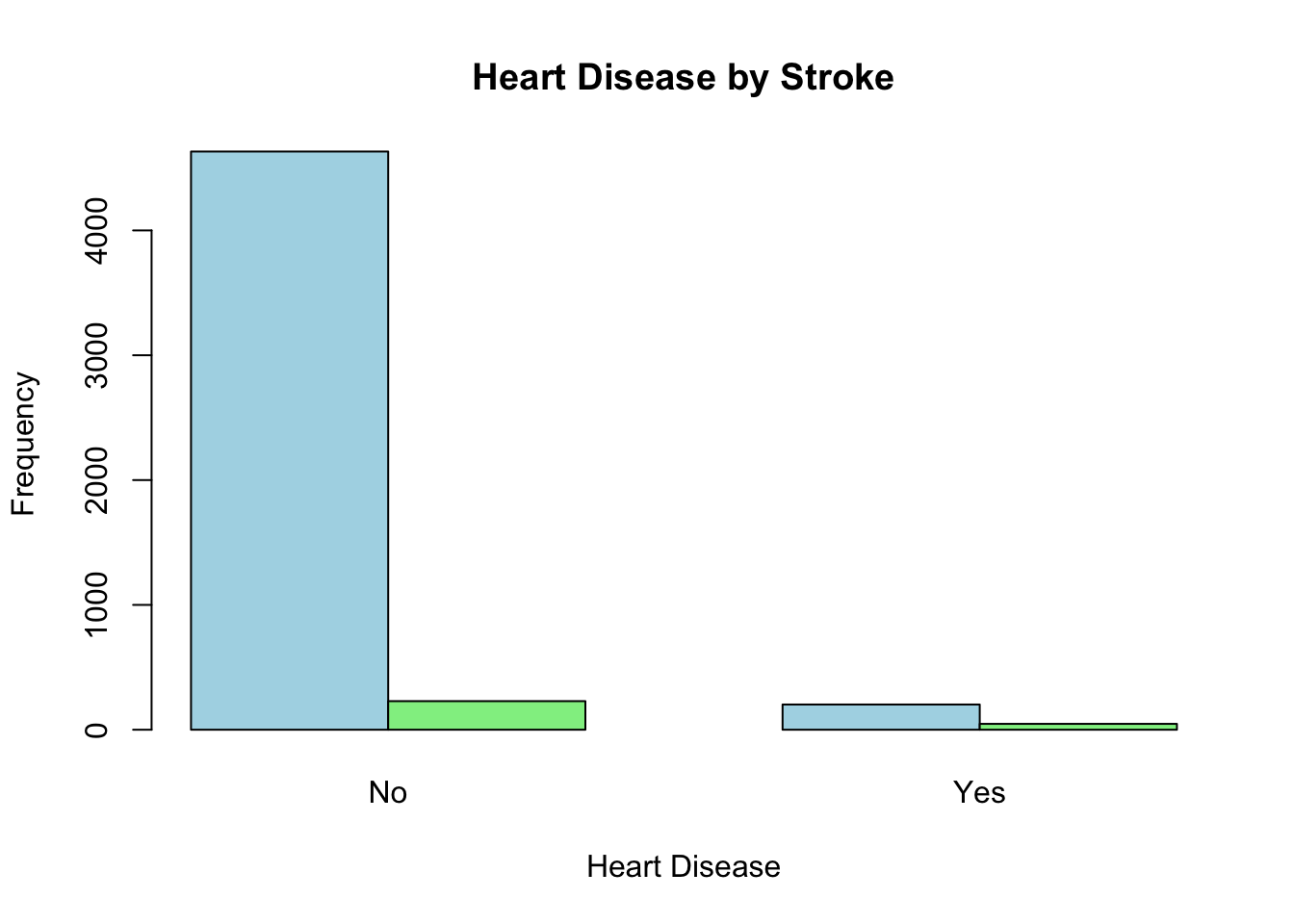
heart_disease: 0 if the patient doesn’t have any heart diseases, 1 if the patient has a heart disease
ever_married: “No” or “Yes”
work_type: “children”, “Govt_jov”, “Never_worked”, “Private” or “Self-employed”
Residence_type: “Rural” or “Urban”
avg_glucose_level: average glucose level in blood
bmi: body mass index
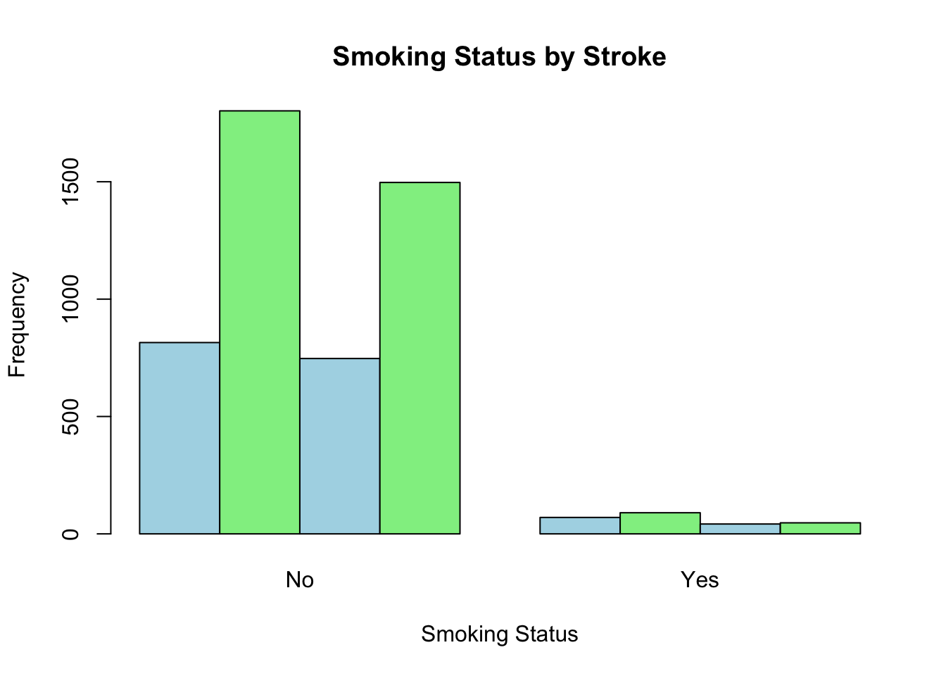
smoking_status: “formerly smoked”, “never smoked”, “smokes” or “Unknown”*
stroke: 1 if the patient had a stroke or 0 if not
Note: “Unknown” in smoking_status means that the information is unavailable for this patient
마지막 열 stroke은 뇌졸중의 유무를 0, 1로 정리했고, 주요 뇌졸중 위험인자들이 정리되어 있다. 결측값은 "N/A" 또는 흡연(smoking_status)인 겅우에는 "Unknown"으로 코딩되어 있는 것을 볼 수 있다. 그리고 문자열로 코딩된 것들은 대부분 R에서는 카테코리형 데이터를 표현하는 팩터(factor)로 되어 있어야 하는데 아직은 원래 값 그대로의 상태로 있다. 우선 이런 것들을 정리해 보자.
ever_married는 결혼 여부로 No, Yes로 되어 있는데 팩터로 바꾼다. work_type는 직업으로 children, Govt_job, Never_worked, Private, Self-employed로 되어 있다. 이것도 팩터로 바꾼다. Residence_type는 거주지로 Rural, Urban으로 되어 있는데, 이것도 팩터로 바꾼다.
이 데이터셋을 다운로드할 수 있다. RDS 파일을 읽을 때는 다음과 같이 readRDS() 함수를 사용하고, 이 데이터프레임의 이름을 지정해 주면 된다.
stroke_df <-readRDS("data/stroke_df.rds")
12.3 기술 통계로 데이터 탐색
이제 정리된 데이터셋을 가지고 기술 통계를 사용하여 데이터를 탐색해 보자.
12.3.1 summary()로 전체적으로 파악하기
개별 변수들을 보기 전에 summary() 함수를 데이터프레임에 적용해 보자. 이 함수는 각 변수의 요약 통계량을 한꺼번에 볼 수 있어서 편리하다. 결과를 관찰해 보면 변수가 숫자형 변수인 경우에는 Minimum, 1st Qu., Median, Mean, 3rd Qu., Maximum이 출력되고, 팩터형 변수인 경우에는 각 레벨의 빈도수가 출력됨을 볼 수 있다.
summary(stroke_df)
      id               gender          age        hypertension heart_disease
 Length:5110        Male  :2115   Min.   : 0.08   No :4612     No :4834
 Class :character   Female:2994   1st Qu.:25.00   Yes: 498     Yes: 276
 Mode  :character   Other :   1   Median :45.00
                                  Mean   :43.23
                                  3rd Qu.:61.00
                                  Max.   :82.00

 ever_married         work_type    residence_type avg_glucose_level
 No :1757     children     : 687   Rural:2514     Min.   : 55.12
 Yes:3353     Govt_job     : 657   Urban:2596     1st Qu.: 77.25
              Never_worked :  22                  Median : 91.89
              Private      :2925                  Mean   :106.15
              Self-employed: 819                  3rd Qu.:114.09
                                                  Max.   :271.74

      bmi                smoking_status stroke
 Min.   :10.30   formerly smoked: 885   No :4861
 1st Qu.:23.50   never smoked   :1892   Yes: 249
 Median :28.10   smokes         : 789
 Mean   :28.89   Unknown        :1544
 3rd Qu.:33.10
 Max.   :97.60
 NA's   :201
이 데이터셋에서 변수는 age, avg_glucose_level, bmi는 숫자형 변수이고, 나머지 변수들은 모두 팩터형 변수이다.
데이터셋의 목적이 뇌졸중의 위험인자를 탐색하는 것일 가능성이 높다. 뇌졸중 여부인 stroke 변수를 기준으로 나머지 변수들을 탐색해 보자
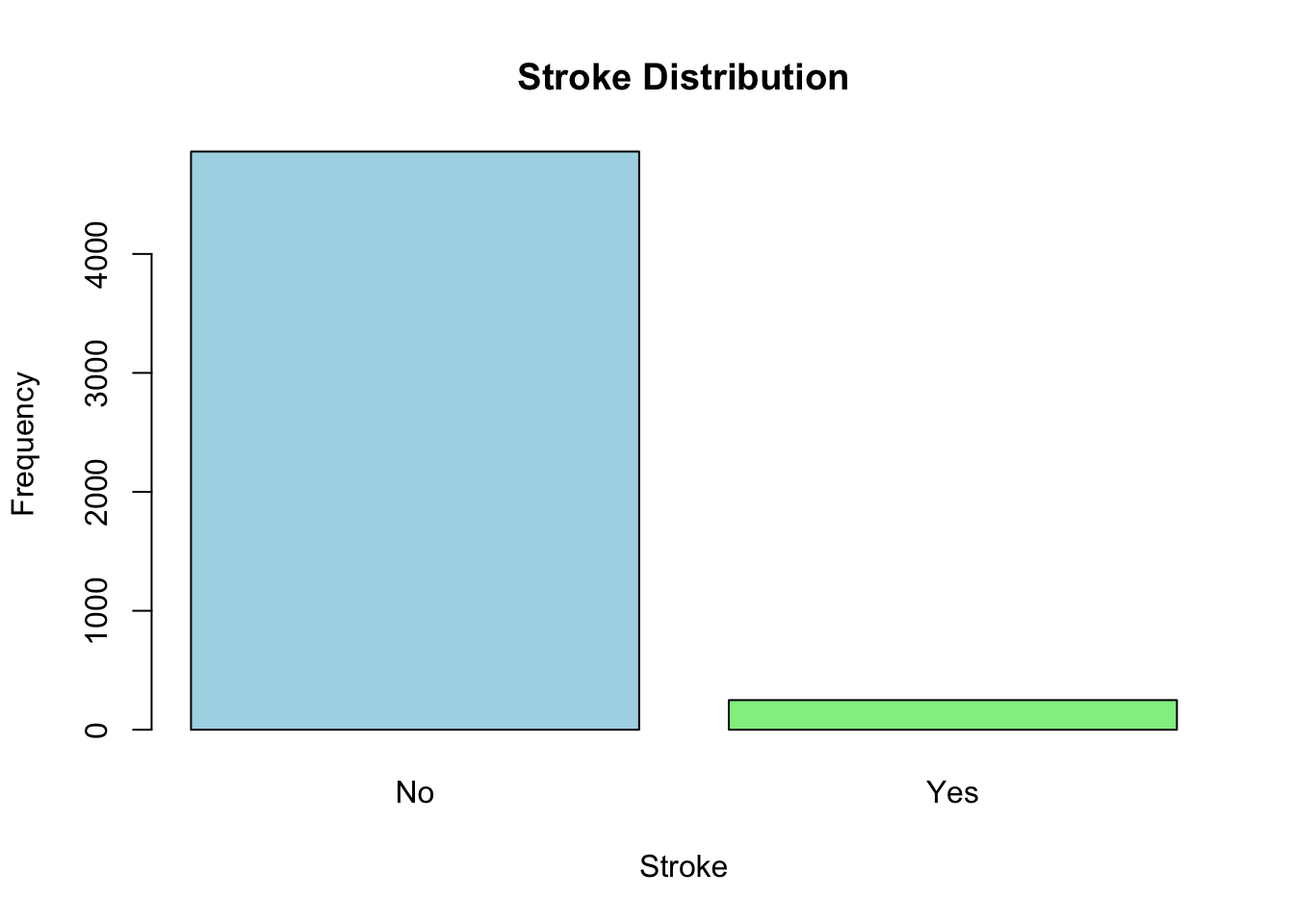
우선 우리의 관심사가 뇌졸중의 유무로 먼저 이 변수를 염두에 두고 시작하는 것이 좋겠다. 전체 5110명 가운데 뇌졸중이 없는 경우가 4861명이고 뇌졸중이 있는 경우가 249명이다.
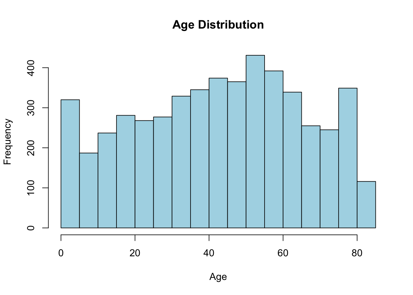
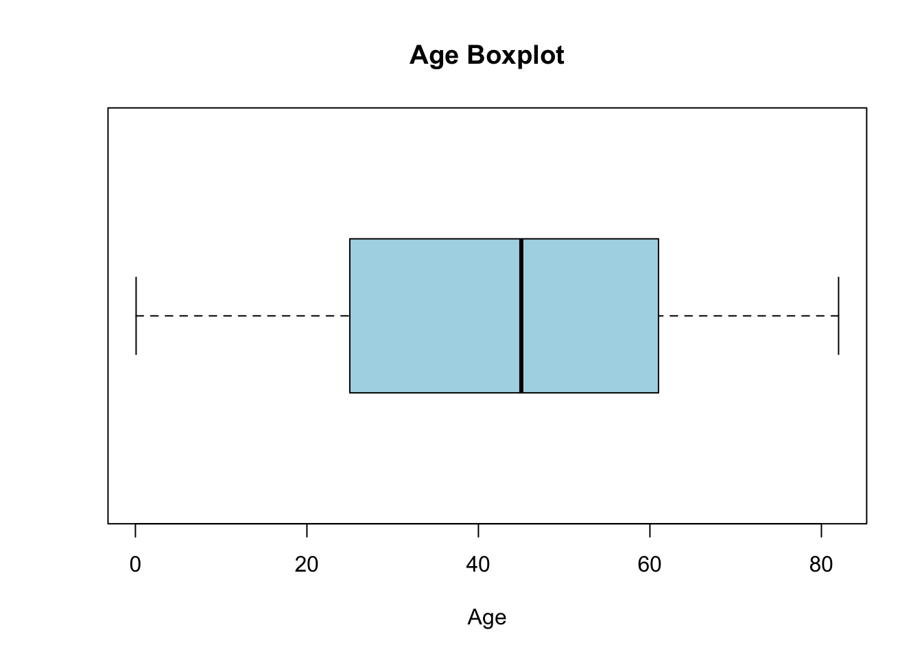
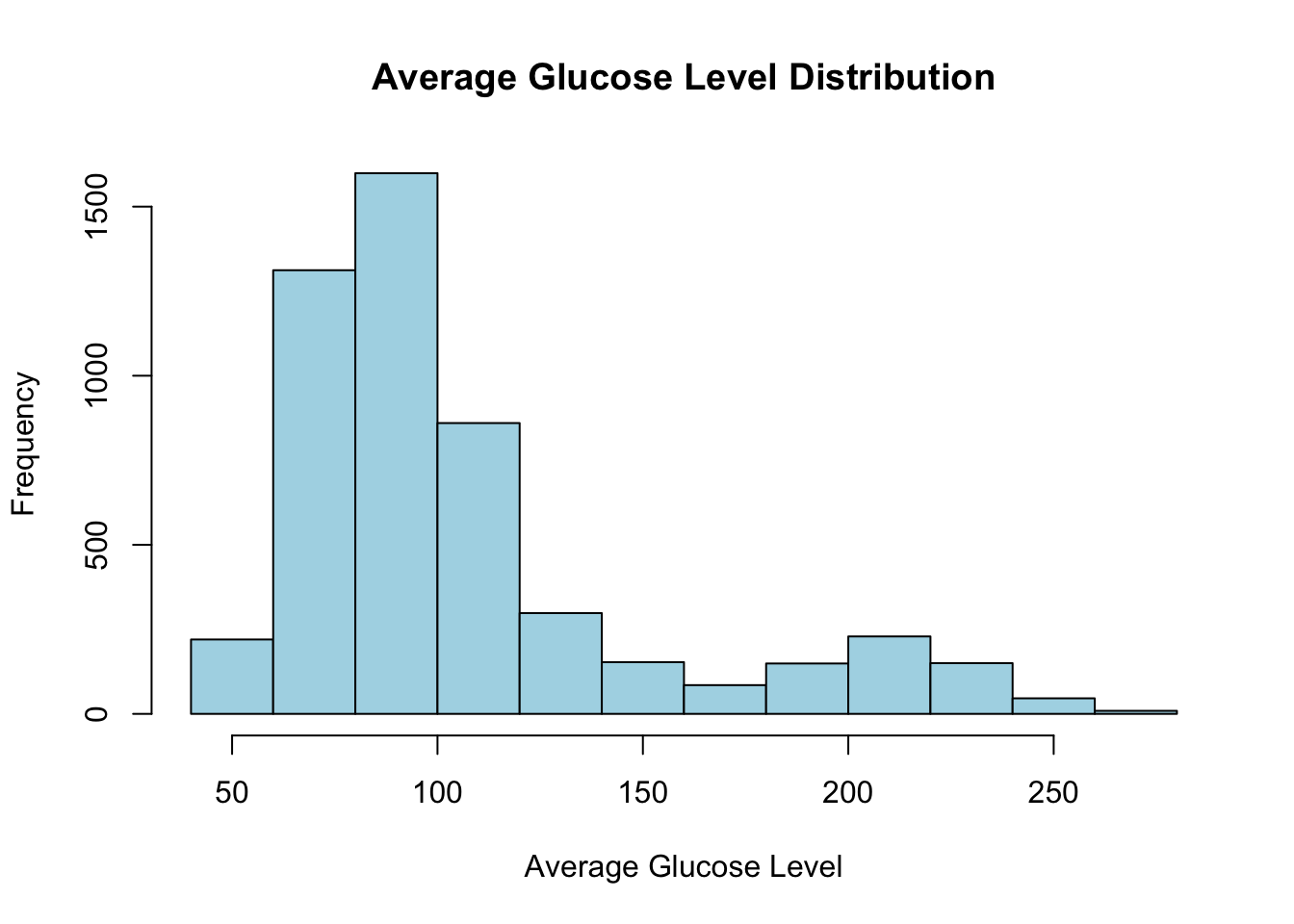
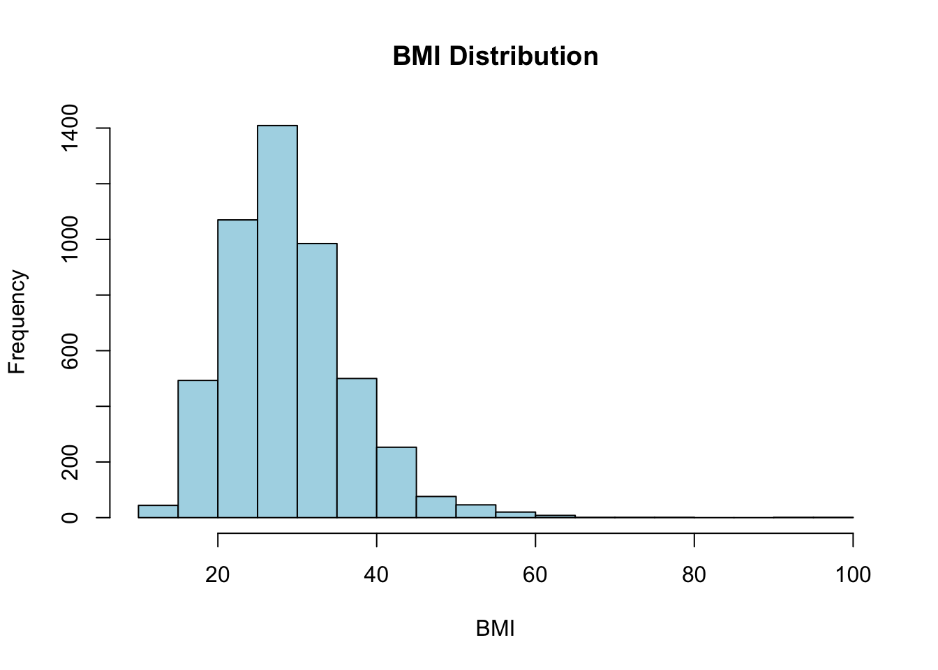
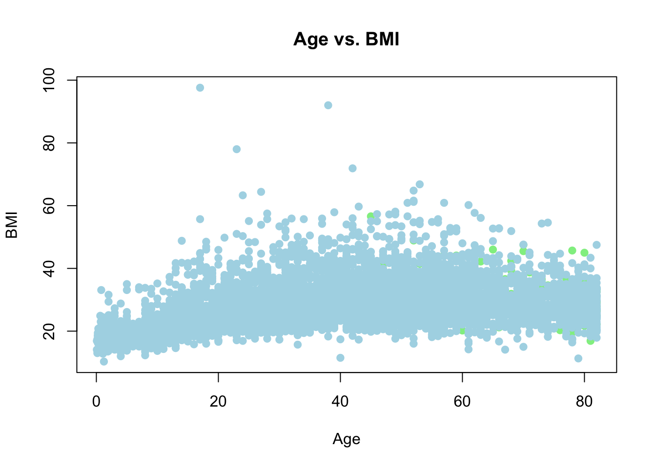
숫자형 변수는 여러 가지 통계량으로 요약할 수 있다. 이 데이터셋에서 숫자형 변수는 age, avg_glucose_level, bmi이다. 이 변수들은 연속형 변수이기 때문에 평균(mean), 분산(var), 표준편차(sd) 등으로 요약할 수 있다. 또 숫자형 변수는 분포가 중요하기 때문에 히스토그램, 박스 플롯, 스캐터 플롯 등으로 정리할 수 있겠다.
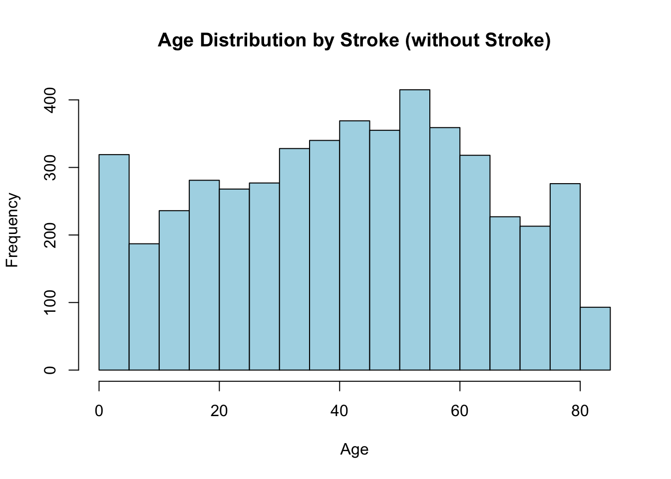
먼저 뇌졸중 여부에 상관없이 전체적으로 보고, 그 다음 뇌졸중의 유무에 따라 어떻게 달라지는지 살펴보자.
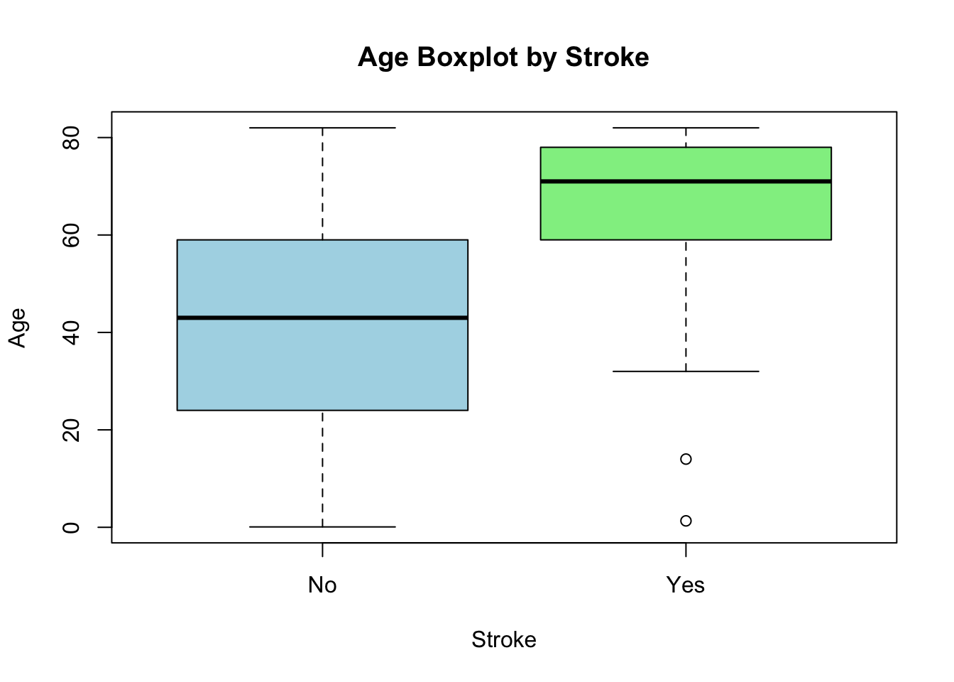
뇌졸중이 있는 그룹과 없는 구룹의 평균 차이가 있는지 t.test()를 사용해 검정해 보았다.
result <-t.test(stroke_df$age[stroke_df$stroke =="No"], stroke_df$age[stroke_df$stroke =="Yes"],var.equal =TRUE)result
    Two Sample t-test

data:  stroke_df$age[stroke_df$stroke == "No"] and stroke_df$age[stroke_df$stroke == "Yes"]
t = -18.081, df = 5108, p-value < 2.2e-16
alternative hypothesis: true difference in means is not equal to 0
95 percent confidence interval:
 -28.54933 -22.96396
sample estimates:
mean of x mean of y
 41.97154  67.72819
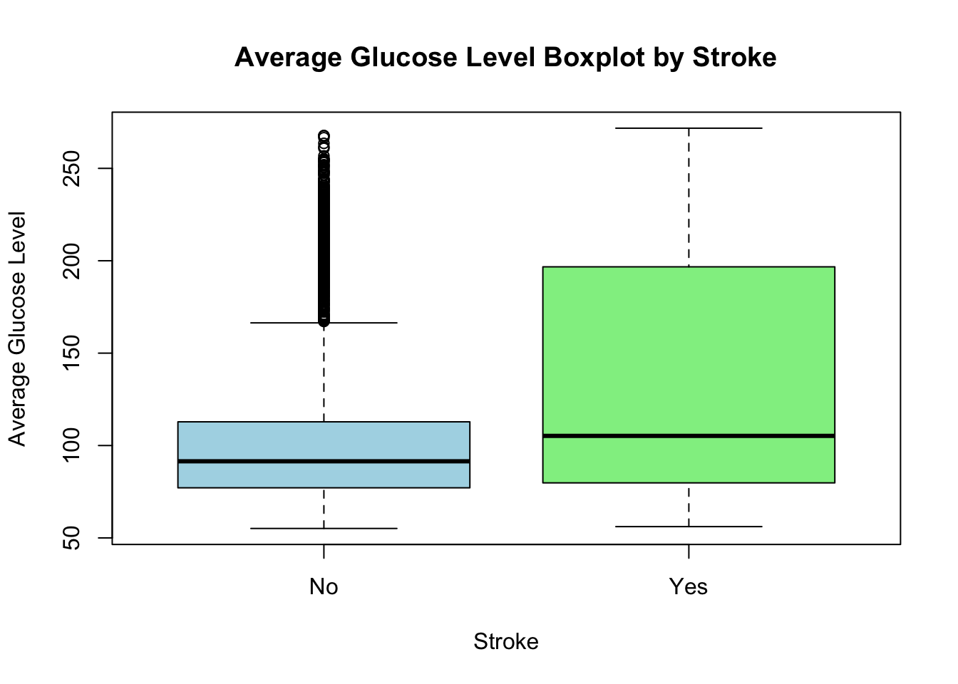
result <-t.test(stroke_df$avg_glucose_level[stroke_df$stroke =="No"], stroke_df$avg_glucose_level[stroke_df$stroke =="Yes"],var.equal =TRUE)result
    Two Sample t-test

data:  stroke_df$avg_glucose_level[stroke_df$stroke == "No"] and stroke_df$avg_glucose_level[stroke_df$stroke == "Yes"]
t = -9.5134, df = 5108, p-value < 2.2e-16
alternative hypothesis: true difference in means is not equal to 0
95 percent confidence interval:
 -33.46754 -22.03091
sample estimates:
mean of x mean of y
 104.7955  132.5447
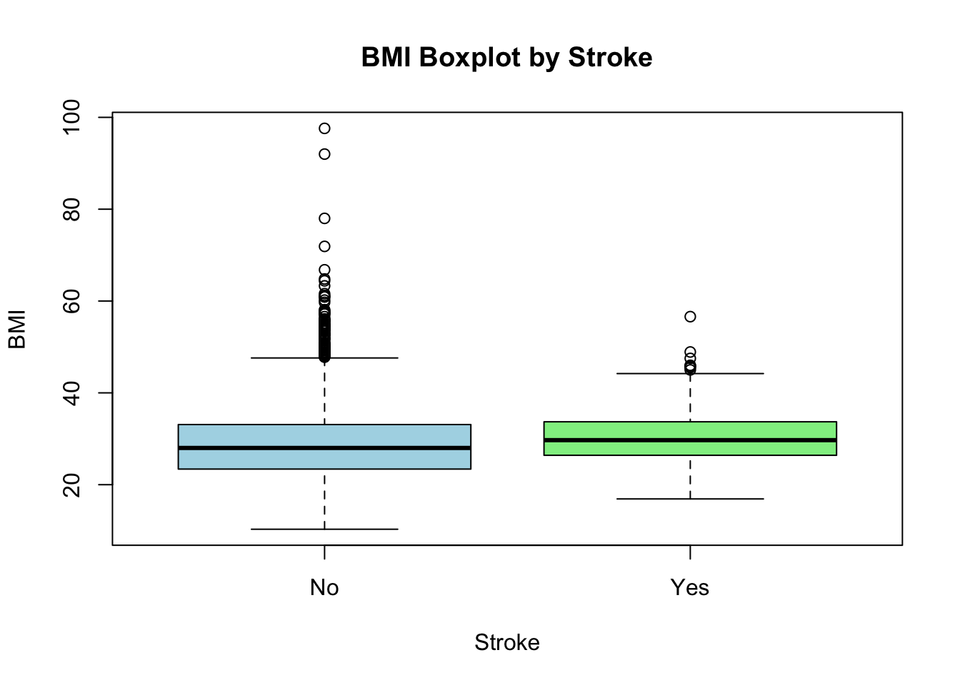
result <-t.test(stroke_df$bmi[stroke_df$stroke =="No"], stroke_df$bmi[stroke_df$stroke =="Yes"],var.equal =TRUE)result
    Two Sample t-test

data:  stroke_df$bmi[stroke_df$stroke == "No"] and stroke_df$bmi[stroke_df$stroke == "Yes"]
t = -2.9709, df = 4907, p-value = 0.002983
alternative hypothesis: true difference in means is not equal to 0
95 percent confidence interval:
 -2.7358507 -0.5606053
sample estimates:
mean of x mean of y
 28.82306  30.47129
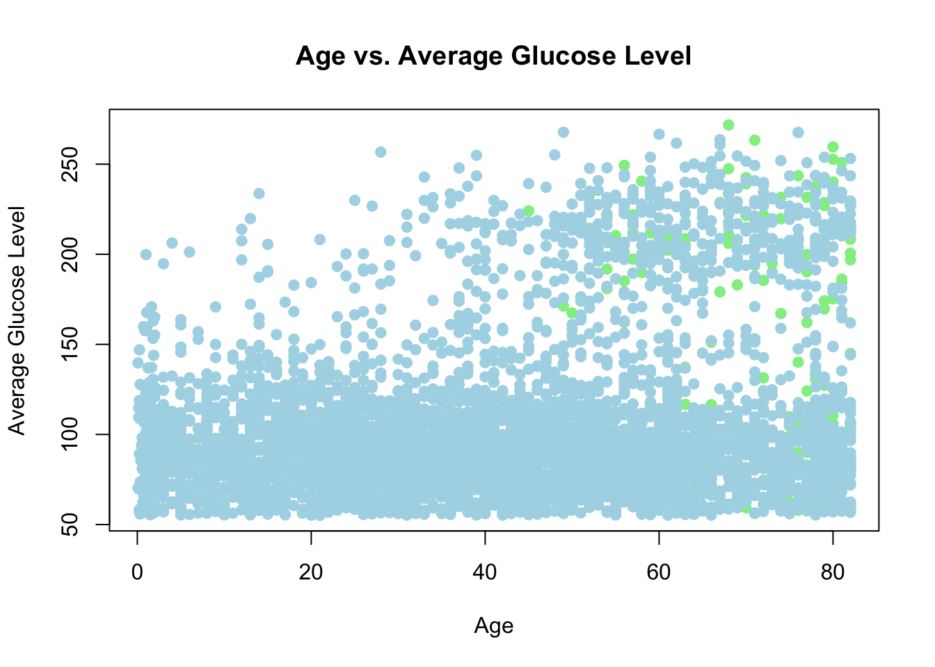
age와 avg_glucose_level의 관계를 스캐터 플롯으로 그려 보자.
plot(stroke_df$age, stroke_df$avg_glucose_level,main ="Age vs. Average Glucose Level",xlab ="Age",ylab ="Average Glucose Level",col =ifelse(stroke_df$stroke =="Yes", "lightgreen", "lightblue"),pch =19)
상관계수를 구해 보자.
cor(stroke_df$age, stroke_df$avg_glucose_level, use ="pairwise.complete.obs")
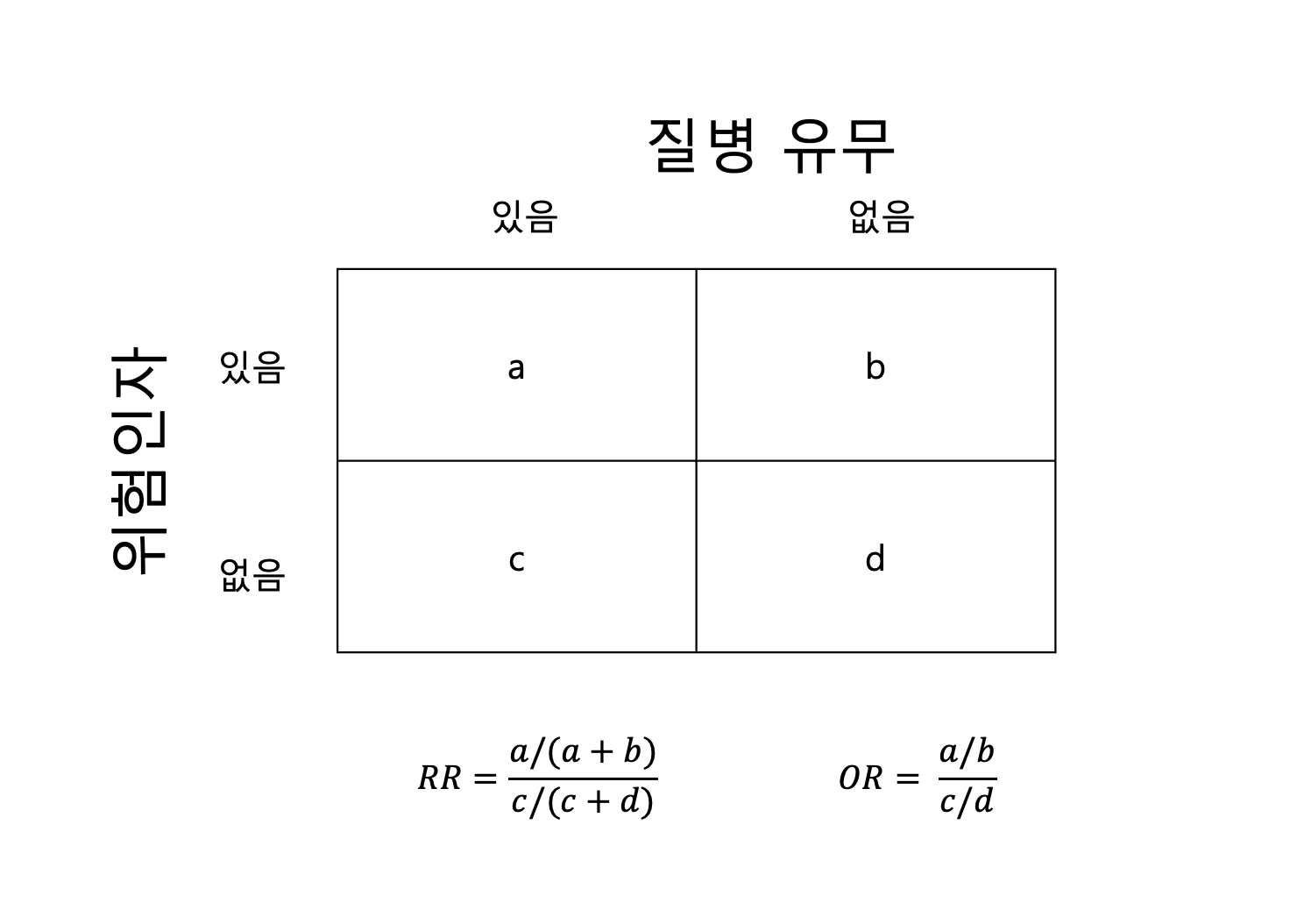
$data

          No Yes Total
  No    4429 183  4612
  Yes    432  66   498
  Total 4861 249  5110

$measure
     risk ratio with 95% C.I.
      estimate   lower upper
  No  1.000000      NA    NA
  Yes 3.340049 2.56046 4.357

$p.value
     two-sided
       midp.exact fisher.exact   chi.square
  No           NA           NA           NA
  Yes 5.77316e-15 4.549182e-15 6.068123e-20

$correction
[1] FALSE

attr(,"method")
[1] "Unconditional MLE & normal approximation (Wald) CI"
oddsratio(tbl)
$data

          No Yes Total
  No    4429 183  4612
  Yes    432  66   498
  Total 4861 249  5110

$measure
     odds ratio with 95% C.I.
      estimate    lower    upper
  No  1.000000       NA       NA
  Yes 3.701246 2.729655 4.964923

$p.value
     two-sided
       midp.exact fisher.exact   chi.square
  No           NA           NA           NA
  Yes 5.77316e-15 4.549182e-15 6.068123e-20

$correction
[1] FALSE

attr(,"method")
[1] "median-unbiased estimate & mid-p exact CI"