# 설치
install.packages("dpylr")
# 로딩
library(dplyr)11 dplyr로 데이터 가공
R dplyr 패키지는 tidyverse를 구성하는 주요 패키지의 하나이며, R 데이터프레임을 가공하여 사용자가 원하는 형태로 변환시키는 기능을 제공한다. 개념과 사용법이 쉽고 또한 기능이 강력하여 R 사용자들이 즐겨 사용하는 도구 가운데 하나이다. d는 data.frame, plyr는 공구(tools)을 의미한다. R dplyr은 파이썬 세계의 팬더스(pandas), 폴라스(polars), SQL 세계의 DuckDB 등과 함께 스프레드시트와 같은 4각형 데이터를 처리하는 핵심 도구로 인정받고 있다. 또 이해를 넓혀 보면 관계형 데이터베이스를 다루는 SQL(structured query language)과도 깊게 연관되어 있으며, SQL을 사용하지 않아도 데이터베이스와도 소통할 수 있다.
![]()
dplyr 설치와 사용은 다음과 같은 방법 가운데 하나를 선택한다. tidyverse를 설치하고 부르면 여기에 포함되어 있어 따로 관리할 필요가 없기도 하다.
또는 다음과 같이 해도 된다.
install.packages("tidyverse")
library("tidyverse")
11.1 도움이 되는 자료
dplyr 패키지는 워낙 인기가 많아 인터넷을 검색하면 수많은 자료를 자료를 찾을 수 있을 것이다. 그래도 가장 읽을 만하다고 보는 문서는 패키지에 내장된 비니에트와 dplyr 저자 등이 설명하는 아래 책의 내용이다.
11.2 dplyr을 시작하기에 앞서 알아둘 내용
dplyr에선 파이프(pipe) 연산자를 많이 사용한다. ( 8 참고) 파이프(pipe)란 수도나 가스관처럼 흐름을 연결하는 구조를 말한다. R에서는 이런 연산자가 native로 지원하는 것이 없어서 처음에는 magrittr이라는 패키지를 통해서 이 기능을 사용했고, %>%라는 연산자를 이용했다. 그러다가 나중에 파이프에 대한 요구가 증가하면서 네이티브로 지원하기 시작했고, |>이라는 연산자를 제공한다. 파이프의 개념은 간단하다. 앞의 연산의 결과가 다음 함수의 첫 번째 인자로 전달된다. 예를 들어, 다음과 같은 코드가 있다고 하자.
Attaching package: 'dplyr'The following objects are masked from 'package:stats':
filter, lagThe following objects are masked from 'package:base':
intersect, setdiff, setequal, union mpg cyl
Mazda RX4 21.0 6
Mazda RX4 Wag 21.0 6
Datsun 710 22.8 4
Hornet 4 Drive 21.4 6
Merc 240D 24.4 4
Merc 230 22.8 4이 코드는 다음과 같은 의미를 갖는다.
위 뒤 코드는 같은 결과를 내지만, 앞의 코드의 가독성이 더 높고, 중간 변수들을 만들지 않아도 되어 메모리로 아끼고 이름들을 관리하지 않아도 된다는 장점을 가진다. 여기서는 R 네이티브 연산자인 |>을 사용한다(%>%를 사용해도 문제가 될 것은 없다).
dplyr를 사용할 때는 non-standard evaluation(NSE)을 사용한다. 이 의미는 별도로 찾아보길 바라고, 단 알아둘 것은 열 이름을 사용할 때 작은따옴표나 큰따옴표 없이 바로 열 이름을 사용한다는 점이다. 이런 점은 R 콘솔에서는 아주 편리하지만 코드로 프로그래밍할 때는 부가적으로 고려해야 하는 점들이 존재한다. 그것은 Programming with dplyr 문서를 참고하길 바란다.
dplyr은 데이터프레임을 처리하는 도구이다 그래서 dplyr의 주요 동사(verbs)는 데이터프레임을 받아서 데이터프레임을 반환한다. 예를 들어, filter() 함수는 데이터프레임을 받아서 데이터프레임을 반환한다. 그래서 대부분 코드는 데이터프레임에서 시작하여 데이터프레임으로 끝난다.
dplyr의 핵심 개발자인 Hadley Wickham은 문법을 좋아한다. 굉장한 인기를 얻은 그래픽 패키지인 ggplot2의 gg는 grammer of graphics의 약자이다. dplyr은 grammer of data manipulation의 약자이다. 그는 어떤 도구의 의미를 부여할 때 문법(grammer)라는 단어를 즐겨 사용한다. dplyr에서는 핵심 함수들을 뭔가를 하는 동사라는 의미에서 verbs라고 부른다.
11.3 dplyr 개론
- 이 글은 dplyr 비니에트 Introduction to dplyr를 요약(주로 번역)한 것임.
패키지를 로딩하고, 그 안에 포함된 starwars 데이터셋을 살펴보자.
# A tibble: 6 × 14
  name      height  mass hair_color skin_color eye_color birth_year sex   gender
  <chr>      <int> <dbl> <chr>      <chr>      <chr>          <dbl> <chr> <chr>
1 Luke Sky…    172    77 blond      fair       blue            19   male  mascu…
2 C-3PO        167    75 <NA>       gold       yellow         112   none  mascu…
3 R2-D2         96    32 <NA>       white, bl… red             33   none  mascu…
4 Darth Va…    202   136 none       white      yellow          41.9 male  mascu…
5 Leia Org…    150    49 brown      light      brown           19   fema… femin…
6 Owen Lars    178   120 brown, gr… light      blue            52   male  mascu…
# ℹ 5 more variables: homeworld <chr>, species <chr>, films <list>,
#   vehicles <list>, starships <list>
11.4 단일 테이블 동사(single table verbs)
먼저 단일 테이블을 대상하는 함수들을 다룬다. 앞에서 설명한 것처럼 이들을 패키지 저자는 single table verbs라고 부른다. 이들 함수를 배울 때는 행과 열 방향을 머릿속에 그리면 좋다.
- 행
- 열
-
select(): 사용할 열들을 선택 -
rename(): 열 이름 변경 -
mutate(): 기존 열들의 값을 가지고 새로운 열을 추가 -
relocate(): 열의 위치 변경
-
- 행 그룹
11.4.1 행을 대상으로 한 함수
11.4.1.1 filter(): 조건에 맞는 행들을 필터링
이 함수에 조건을 주면, 조건을 만족하는 행들을 걸러낸댜.
다음은 skin_color가 "light"이고(AND), eye_color가 "brown" 값을 가지는 행들을 걸러낸다.
starwars |> filter(skin_color == "light", eye_color == "brown")# A tibble: 7 × 14
name height mass hair_color skin_color eye_color birth_year sex gender
<chr> <int> <dbl> <chr> <chr> <chr> <dbl> <chr> <chr>
1 Leia Org… 150 49 brown light brown 19 fema… femin…
2 Biggs Da… 183 84 black light brown 24 male mascu…
3 Padmé Am… 185 45 brown light brown 46 fema… femin…
4 Cordé 157 NA brown light brown NA <NA> <NA>
5 Dormé 165 NA brown light brown NA fema… femin…
6 Raymus A… 188 79 brown light brown NA male mascu…
7 Poe Dame… NA NA brown light brown NA male mascu…
# ℹ 5 more variables: homeworld <chr>, species <chr>, films <list>,
# vehicles <list>, starships <list>
11.4.1.2 arrange(): 정렬 (행들의 위치 변경)
arrange() 함수 안에는 정렬의 기준이 되는 열을 순서대로 지정한다.
starwars |> arrange(height, mass)# A tibble: 87 × 14
name height mass hair_color skin_color eye_color birth_year sex gender
<chr> <int> <dbl> <chr> <chr> <chr> <dbl> <chr> <chr>
1 Yoda 66 17 white green brown 896 male mascu…
2 Ratts T… 79 15 none grey, blue unknown NA male mascu…
3 Wicket … 88 20 brown brown brown 8 male mascu…
4 Dud Bolt 94 45 none blue, grey yellow NA male mascu…
5 R2-D2 96 32 <NA> white, bl… red 33 none mascu…
6 R4-P17 96 NA none silver, r… red, blue NA none femin…
7 R5-D4 97 32 <NA> white, red red NA none mascu…
8 Sebulba 112 40 none grey, red orange NA male mascu…
9 Gasgano 122 NA none white, bl… black NA male mascu…
10 Watto 137 NA black blue, grey yellow NA male mascu…
# ℹ 77 more rows
# ℹ 5 more variables: homeworld <chr>, species <chr>, films <list>,
# vehicles <list>, starships <list>디폴트는 오름차순이다. 내림차순으로 정렬할 때는 desc() 함수로 감싼다.
# A tibble: 87 × 14
   name     height  mass hair_color skin_color eye_color birth_year sex   gender
   <chr>     <int> <dbl> <chr>      <chr>      <chr>          <dbl> <chr> <chr>
 1 Yarael …    264    NA none       white      yellow          NA   male  mascu…
 2 Tarfful     234   136 brown      brown      blue            NA   male  mascu…
 3 Lama Su     229    88 none       grey       black           NA   male  mascu…
 4 Chewbac…    228   112 brown      unknown    blue           200   male  mascu…
 5 Roos Ta…    224    82 none       grey       orange          NA   male  mascu…
 6 Grievous    216   159 none       brown, wh… green, y…       NA   male  mascu…
 7 Taun We     213    NA none       grey       black           NA   fema… femin…
 8 Rugor N…    206    NA none       green      orange          NA   male  mascu…
 9 Tion Me…    206    80 none       grey       black           NA   male  mascu…
10 Darth V…    202   136 none       white      yellow          41.9 male  mascu…
# ℹ 77 more rows
# ℹ 5 more variables: homeworld <chr>, species <chr>, films <list>,
#   vehicles <list>, starships <list>
11.4.1.3 slice(): 인덱스를 가지고 일부 행들을 선택
위치 값을 가지고 행들을 처리한다.
# 5번째에서 10번째 행을 잘라낸다.
starwars |> slice(5:10)
# A tibble: 6 × 14
name height mass hair_color skin_color eye_color birth_year sex gender
<chr> <int> <dbl> <chr> <chr> <chr> <dbl> <chr> <chr>
1 Leia Org… 150 49 brown light brown 19 fema… femin…
2 Owen Lars 178 120 brown, gr… light blue 52 male mascu…
3 Beru Whi… 165 75 brown light blue 47 fema… femin…
4 R5-D4 97 32 <NA> white, red red NA none mascu…
5 Biggs Da… 183 84 black light brown 24 male mascu…
6 Obi-Wan … 182 77 auburn, w… fair blue-gray 57 male mascu…
# ℹ 5 more variables: homeworld <chr>, species <chr>, films <list>,
# vehicles <list>, starships <list>비슷한 함수로 slice_head(), slice_tail()는 앞부분, 뒷부분을 잘라낸다.
starwars |> slice_head(n = 3)# A tibble: 3 × 14
name height mass hair_color skin_color eye_color birth_year sex gender
<chr> <int> <dbl> <chr> <chr> <chr> <dbl> <chr> <chr>
1 Luke Sky… 172 77 blond fair blue 19 male mascu…
2 C-3PO 167 75 <NA> gold yellow 112 none mascu…
3 R2-D2 96 32 <NA> white, bl… red 33 none mascu…
# ℹ 5 more variables: homeworld <chr>, species <chr>, films <list>,
# vehicles <list>, starships <list>slice_sample() 함수는 무작위로 n개 행을 추출하거나 prop 비율 만큼 추출한다. 부트스트랩(bootstrap)을 수행할 때는 “복원추출”을 사용하는데, 이런 경우에는 replace = TRUE 옵션을 사용한다.
starwars |> slice_sample(n = 5)# A tibble: 5 × 14
name height mass hair_color skin_color eye_color birth_year sex gender
<chr> <int> <dbl> <chr> <chr> <chr> <dbl> <chr> <chr>
1 Palpatine 170 75 grey pale yellow 82 male mascu…
2 Wilhuff … 180 NA auburn, g… fair blue 64 male mascu…
3 Bossk 190 113 none green red 53 male mascu…
4 Raymus A… 188 79 brown light brown NA male mascu…
5 Obi-Wan … 182 77 auburn, w… fair blue-gray 57 male mascu…
# ℹ 5 more variables: homeworld <chr>, species <chr>, films <list>,
# vehicles <list>, starships <list>starwars |> slice_sample(prop = 0.1)# A tibble: 8 × 14
name height mass hair_color skin_color eye_color birth_year sex gender
<chr> <int> <dbl> <chr> <chr> <chr> <dbl> <chr> <chr>
1 Sly Moore 178 48 none pale white NA <NA> <NA>
2 Bossk 190 113 none green red 53 male mascu…
3 Poe Dame… NA NA brown light brown NA male mascu…
4 Greedo 173 74 <NA> green black 44 male mascu…
5 Jabba De… 175 1358 <NA> green-tan… orange 600 herm… mascu…
6 Nien Nunb 160 68 none grey black NA male mascu…
7 Rugor Na… 206 NA none green orange NA male mascu…
8 Saesee T… 188 NA none pale orange NA male mascu…
# ℹ 5 more variables: homeworld <chr>, species <chr>, films <list>,
# vehicles <list>, starships <list>starwars |> slice_sample(prop = 0.1, replace = TRUE)# A tibble: 8 × 14
name height mass hair_color skin_color eye_color birth_year sex gender
<chr> <int> <dbl> <chr> <chr> <chr> <dbl> <chr> <chr>
1 Bossk 190 113 none green red 53 male mascu…
2 Ayla Sec… 178 55 none blue hazel 48 fema… femin…
3 Quarsh P… 183 NA black dark brown 62 male mascu…
4 Quarsh P… 183 NA black dark brown 62 male mascu…
5 Taun We 213 NA none grey black NA fema… femin…
6 Biggs Da… 183 84 black light brown 24 male mascu…
7 Wicket S… 88 20 brown brown brown 8 male mascu…
8 Darth Va… 202 136 none white yellow 41.9 male mascu…
# ℹ 5 more variables: homeworld <chr>, species <chr>, films <list>,
# vehicles <list>, starships <list>slice_min(), slice_max()는 어떤 변수의 최소, 최대값을 가지는 행들을 골라낸다.
# A tibble: 3 × 14
  name      height  mass hair_color skin_color eye_color birth_year sex   gender
  <chr>      <int> <dbl> <chr>      <chr>      <chr>          <dbl> <chr> <chr>
1 Yarael P…    264    NA none       white      yellow            NA male  mascu…
2 Tarfful      234   136 brown      brown      blue              NA male  mascu…
3 Lama Su      229    88 none       grey       black             NA male  mascu…
# ℹ 5 more variables: homeworld <chr>, species <chr>, films <list>,
# vehicles <list>, starships <list># A tibble: 3 × 14
name height mass hair_color skin_color eye_color birth_year sex gender
<chr> <int> <dbl> <chr> <chr> <chr> <dbl> <chr> <chr>
1 Yoda 66 17 white green brown 896 male mascu…
2 Ratts Ty… 79 15 none grey, blue unknown NA male mascu…
3 Wicket S… 88 20 brown brown brown 8 male mascu…
# ℹ 5 more variables: homeworld <chr>, species <chr>, films <list>,
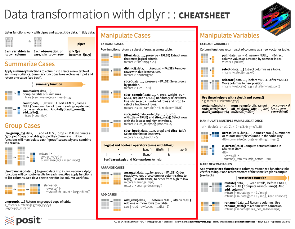
# vehicles <list>, starships <list>이상은 `dplyr cheatsheet에서 다음 내용을 설명한 것이다.
11.4.2 열을 대상으로 하는 함수
select() 함수는 관심이 되는 열들만 골라낸다. 이 함수 안에서는 아주 다양한 방식의 열 선택 방법을 구사할 수 있다.
- 정수: 열의 인덱스
- 열 이름들: 해당 열들
-
:: 데이터프레임에서 맞붙어 있는 변수들 선택 -
!: 해당되지 않는 변수 선택(논리적으로 NOT) -
ends_with(),starts_with(),contains()등 보조 함수 where(참또는거짓반환하는 함수)
starwars |> select(hair_color, skin_color, eye_color)# A tibble: 87 × 3
hair_color skin_color eye_color
<chr> <chr> <chr>
1 blond fair blue
2 <NA> gold yellow
3 <NA> white, blue red
4 none white yellow
5 brown light brown
6 brown, grey light blue
7 brown light blue
8 <NA> white, red red
9 black light brown
10 auburn, white fair blue-gray
# ℹ 77 more rowsstarwars |> select(hair_color:eye_color)# A tibble: 87 × 3
hair_color skin_color eye_color
<chr> <chr> <chr>
1 blond fair blue
2 <NA> gold yellow
3 <NA> white, blue red
4 none white yellow
5 brown light brown
6 brown, grey light blue
7 brown light blue
8 <NA> white, red red
9 black light brown
10 auburn, white fair blue-gray
# ℹ 77 more rowsstarwars |> select(!(hair_color:eye_color))# A tibble: 87 × 11
name height mass birth_year sex gender homeworld species films vehicles
<chr> <int> <dbl> <dbl> <chr> <chr> <chr> <chr> <lis> <list>
1 Luke S… 172 77 19 male mascu… Tatooine Human <chr> <chr>
2 C-3PO 167 75 112 none mascu… Tatooine Droid <chr> <chr>
3 R2-D2 96 32 33 none mascu… Naboo Droid <chr> <chr>
4 Darth … 202 136 41.9 male mascu… Tatooine Human <chr> <chr>
5 Leia O… 150 49 19 fema… femin… Alderaan Human <chr> <chr>
6 Owen L… 178 120 52 male mascu… Tatooine Human <chr> <chr>
7 Beru W… 165 75 47 fema… femin… Tatooine Human <chr> <chr>
8 R5-D4 97 32 NA none mascu… Tatooine Droid <chr> <chr>
9 Biggs … 183 84 24 male mascu… Tatooine Human <chr> <chr>
10 Obi-Wa… 182 77 57 male mascu… Stewjon Human <chr> <chr>
# ℹ 77 more rows
# ℹ 1 more variable: starships <list># A tibble: 87 × 3
hair_color skin_color eye_color
<chr> <chr> <chr>
1 blond fair blue
2 <NA> gold yellow
3 <NA> white, blue red
4 none white yellow
5 brown light brown
6 brown, grey light blue
7 brown light blue
8 <NA> white, red red
9 black light brown
10 auburn, white fair blue-gray
# ℹ 77 more rows
11.4.2.1 rename() 함수
rename() 함수는 열의 이름을 바꾼다. 새로운이름 = 이전이름 형태로 인자를 지정한다.
starwars |> rename(Name = name)# A tibble: 87 × 14
Name height mass hair_color skin_color eye_color birth_year sex gender
<chr> <int> <dbl> <chr> <chr> <chr> <dbl> <chr> <chr>
1 Luke Sk… 172 77 blond fair blue 19 male mascu…
2 C-3PO 167 75 <NA> gold yellow 112 none mascu…
3 R2-D2 96 32 <NA> white, bl… red 33 none mascu…
4 Darth V… 202 136 none white yellow 41.9 male mascu…
5 Leia Or… 150 49 brown light brown 19 fema… femin…
6 Owen La… 178 120 brown, gr… light blue 52 male mascu…
7 Beru Wh… 165 75 brown light blue 47 fema… femin…
8 R5-D4 97 32 <NA> white, red red NA none mascu…
9 Biggs D… 183 84 black light brown 24 male mascu…
10 Obi-Wan… 182 77 auburn, w… fair blue-gray 57 male mascu…
# ℹ 77 more rows
# ℹ 5 more variables: homeworld <chr>, species <chr>, films <list>,
# vehicles <list>, starships <list>
11.4.2.2 mutate(): 새로운 열 추가
mutate() 함수는 보통 기존 열에 있는 값들을 계산하여 새로운 열을 만들면서 추가한 데이터프레임을 반환한다.
starwars |> mutate(height_m = height / 100)# A tibble: 87 × 15
name height mass hair_color skin_color eye_color birth_year sex gender
<chr> <int> <dbl> <chr> <chr> <chr> <dbl> <chr> <chr>
1 Luke Sk… 172 77 blond fair blue 19 male mascu…
2 C-3PO 167 75 <NA> gold yellow 112 none mascu…
3 R2-D2 96 32 <NA> white, bl… red 33 none mascu…
4 Darth V… 202 136 none white yellow 41.9 male mascu…
5 Leia Or… 150 49 brown light brown 19 fema… femin…
6 Owen La… 178 120 brown, gr… light blue 52 male mascu…
7 Beru Wh… 165 75 brown light blue 47 fema… femin…
8 R5-D4 97 32 <NA> white, red red NA none mascu…
9 Biggs D… 183 84 black light brown 24 male mascu…
10 Obi-Wan… 182 77 auburn, w… fair blue-gray 57 male mascu…
# ℹ 77 more rows
# ℹ 6 more variables: homeworld <chr>, species <chr>, films <list>,
# vehicles <list>, starships <list>, height_m <dbl>만약 새롭게 만든 열만을 남기고자 할 경우(이 열만 가진 데이터프레임을 만듦), .keep = "none" 옵션을 사용한다.
starwars |>
    mutate(
        height_m = height / 100,
        BMI = mass / (height_m^2),
        .keep = "none"
    )
# A tibble: 87 × 2
height_m BMI
<dbl> <dbl>
1 1.72 26.0
2 1.67 26.9
3 0.96 34.7
4 2.02 33.3
5 1.5 21.8
6 1.78 37.9
7 1.65 27.5
8 0.97 34.0
9 1.83 25.1
10 1.82 23.2
# ℹ 77 more rows
11.4.2.3 relocate(): 열의 위치를 재조정
relocate() 함수는 열의 위치를 재조정할 때 사용한다. .after, .before라는 인자를 사용한다.
다음은 sex에서 homeworld까지의 열들을 height 열 앞으로 옮긴다.
starwars |> relocate(sex:homeworld, .before = height)# A tibble: 87 × 14
name sex gender homeworld height mass hair_color skin_color eye_color
<chr> <chr> <chr> <chr> <int> <dbl> <chr> <chr> <chr>
1 Luke Sky… male mascu… Tatooine 172 77 blond fair blue
2 C-3PO none mascu… Tatooine 167 75 <NA> gold yellow
3 R2-D2 none mascu… Naboo 96 32 <NA> white, bl… red
4 Darth Va… male mascu… Tatooine 202 136 none white yellow
5 Leia Org… fema… femin… Alderaan 150 49 brown light brown
6 Owen Lars male mascu… Tatooine 178 120 brown, gr… light blue
7 Beru Whi… fema… femin… Tatooine 165 75 brown light blue
8 R5-D4 none mascu… Tatooine 97 32 <NA> white, red red
9 Biggs Da… male mascu… Tatooine 183 84 black light brown
10 Obi-Wan … male mascu… Stewjon 182 77 auburn, w… fair blue-gray
# ℹ 77 more rows
# ℹ 5 more variables: birth_year <dbl>, species <chr>, films <list>,
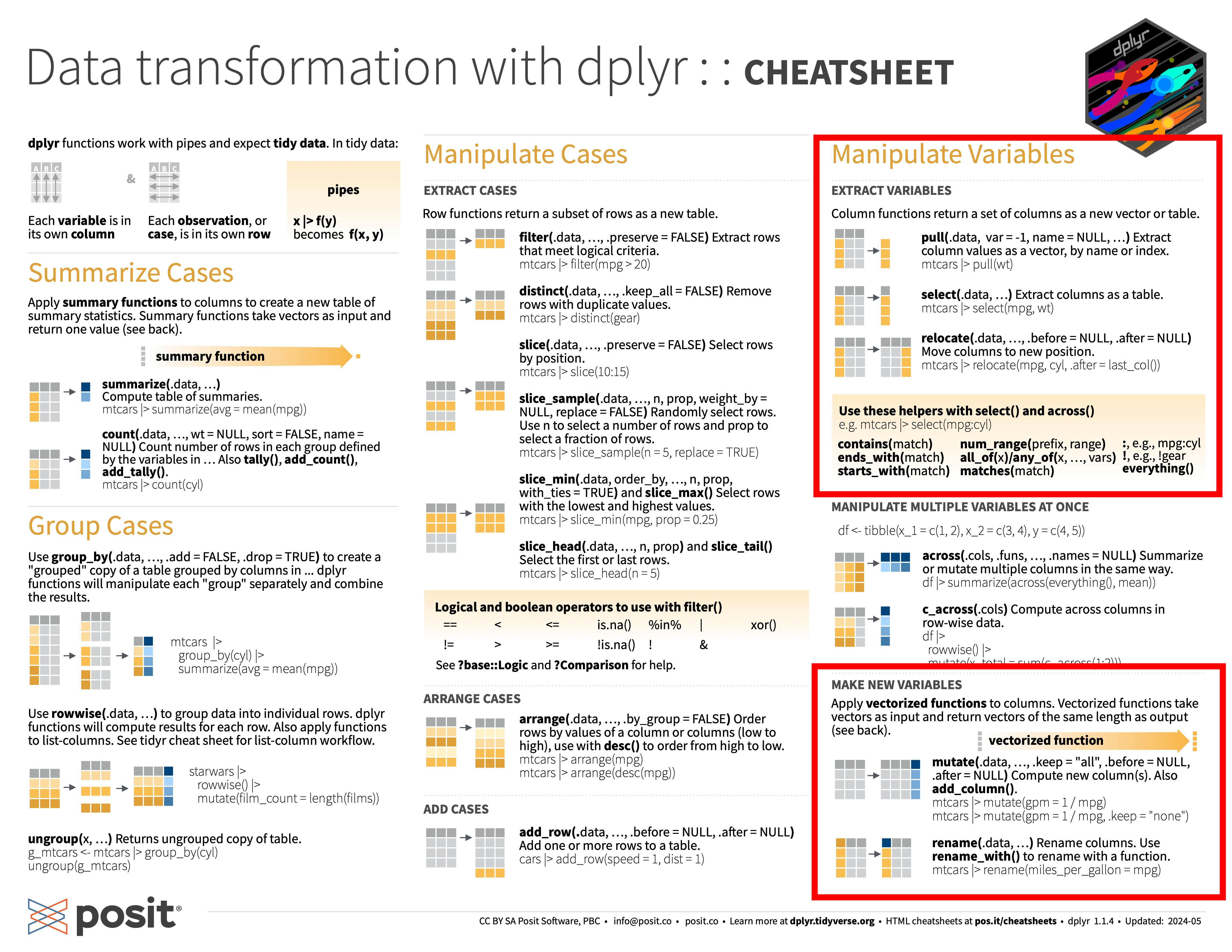
# vehicles <list>, starships <list>이상은 dplyr cheatsheet에서 다음 내용을 정리한 셈이다.
11.4.3 행 그룹에 대한 써머리: summarise() 함수
이 함수는 하나의 데이터프레임을 통계 계산을 통해 한 줄로 요약할 때 편리하다. 나중에 group_by()와 함께 사용할 때, 그룹별 차이를 정리하여 볼 때 편리하다.
11.5 그룹화 데이터
- 이 글은
dplyr비니에트 [Grouped Data](https://dplyr.tidyverse.org/articles/grouping.html과 함께 읽으면 도움일 될 것임.
11.5.1 group_by() 함수로 그룹화 데이터프레임 만들기
보통 카테고리형 변수(치료군/대조군 등)을 사용하는 이유는 이 변수의 레벨에 따라 데이터셋을 분리하여 그 특징들을 서로 비교하려는 것이다. 여기서 말하는 그룹화 데이터프레임이란 논리적으로 전체 데이터셋을 분리한 데이터셋을 말한다.
- 그룹화 변수를
group_by()함수로 넘기면 그룹화된 데이터프레임이 만들어 진다.
출력하면 그룹화된 데이터프레임인지 알 수 있다. Tibble인 경우 2번째 행에 Groups:로 시작되는 행을 볼 수 있다.
by_species# A tibble: 87 × 14
# Groups: species [38]
name height mass hair_color skin_color eye_color birth_year sex gender
<chr> <int> <dbl> <chr> <chr> <chr> <dbl> <chr> <chr>
1 Luke Sk… 172 77 blond fair blue 19 male mascu…
2 C-3PO 167 75 <NA> gold yellow 112 none mascu…
3 R2-D2 96 32 <NA> white, bl… red 33 none mascu…
4 Darth V… 202 136 none white yellow 41.9 male mascu…
5 Leia Or… 150 49 brown light brown 19 fema… femin…
6 Owen La… 178 120 brown, gr… light blue 52 male mascu…
7 Beru Wh… 165 75 brown light blue 47 fema… femin…
8 R5-D4 97 32 <NA> white, red red NA none mascu…
9 Biggs D… 183 84 black light brown 24 male mascu…
10 Obi-Wan… 182 77 auburn, w… fair blue-gray 57 male mascu…
# ℹ 77 more rows
# ℹ 5 more variables: homeworld <chr>, species <chr>, films <list>,
# vehicles <list>, starships <list>by_sex_gender# A tibble: 87 × 14
# Groups: sex, gender [6]
name height mass hair_color skin_color eye_color birth_year sex gender
<chr> <int> <dbl> <chr> <chr> <chr> <dbl> <chr> <chr>
1 Luke Sk… 172 77 blond fair blue 19 male mascu…
2 C-3PO 167 75 <NA> gold yellow 112 none mascu…
3 R2-D2 96 32 <NA> white, bl… red 33 none mascu…
4 Darth V… 202 136 none white yellow 41.9 male mascu…
5 Leia Or… 150 49 brown light brown 19 fema… femin…
6 Owen La… 178 120 brown, gr… light blue 52 male mascu…
7 Beru Wh… 165 75 brown light blue 47 fema… femin…
8 R5-D4 97 32 <NA> white, red red NA none mascu…
9 Biggs D… 183 84 black light brown 24 male mascu…
10 Obi-Wan… 182 77 auburn, w… fair blue-gray 57 male mascu…
# ℹ 77 more rows
# ℹ 5 more variables: homeworld <chr>, species <chr>, films <list>,
# vehicles <list>, starships <list>-
group_keys()함수를 사용하여, 각 그룹의 키를 확인할 수 있다. 즉 그룹이 나눠지는 기준 값이 무엇인지를 알 수 있다.
by_species |> group_keys()# A tibble: 38 × 1
species
<chr>
1 Aleena
2 Besalisk
3 Cerean
4 Chagrian
5 Clawdite
6 Droid
7 Dug
8 Ewok
9 Geonosian
10 Gungan
# ℹ 28 more rowsby_sex_gender |> group_keys()# A tibble: 6 × 2
sex gender
<chr> <chr>
1 female feminine
2 hermaphroditic masculine
3 male masculine
4 none feminine
5 none masculine
6 <NA> <NA> -
group_indices()함수를 통해서 행이 어떤 그룹에 속하는지 알 수 있다.
by_species |> group_indices() [1] 11 6 6 11 11 11 11 6 11 11 11 11 34 11 24 12 11 38 36 11 11 6 31 11 11
[26] 18 11 11 8 26 11 21 11 11 10 10 10 11 30 7 11 11 37 32 32 1 33 35 29 11
[51] 3 20 37 27 13 23 16 4 38 38 11 9 17 17 11 11 11 11 5 2 15 15 11 6 25
[76] 19 28 14 34 11 38 22 11 11 11 6 11-
group_rows()함수로 각 그룹을 구성하는 행들을 알 수 있다.
by_sex_gender |> group_rows()<list_of<integer>[6]>
[[1]]
[1] 5 7 27 34 42 45 54 63 64 65 69 72 73 77 84 87
[[2]]
[1] 16
[[3]]
[1] 1 4 6 9 10 11 12 13 14 15 17 19 20 21 23 24 25 26 28 29 30 31 32 33 35
[26] 36 37 38 39 40 41 43 44 46 47 48 49 50 51 52 53 55 56 57 58 61 62 66 67 68
[51] 70 71 75 76 78 79 80 82 83 85
[[4]]
[1] 74
[[5]]
[1] 2 3 8 22 86
[[6]]
[1] 18 59 60 81-
group_vars()를 통해서 그룹핑 변수 이름을 확인한다.
- (이미) 그룹화된 데이터프레임에 대하여
group_by()함수를 적용하면 기존 그룹핑이 해제되고 새로운 변수에 따라 다시 그룹핑된다. 이렇게 새롭게 그륩핑하는 것이 아니라 추가하려고 하면.add = TRUE인자를 사용한다. 그룹핑을 해제하려면ungroup()함수를 사용한다.
그룹화 데이터프레임을 사용하면 다음과 같이 그룹에 대한 써머리를 한 문장으로 간결하게 정리할 수 있다.
starwars |>
    group_by(sex) |>
    summarise(N = n(), mean_height = mean(height, na.rm = TRUE)) |>
knitr::kable()| sex | N | mean_height |
|---|---|---|
| female | 16 | 171.5714 |
| hermaphroditic | 1 | 175.0000 |
| male | 60 | 179.1228 |
| none | 6 | 131.2000 |
| NA | 4 | 175.0000 |
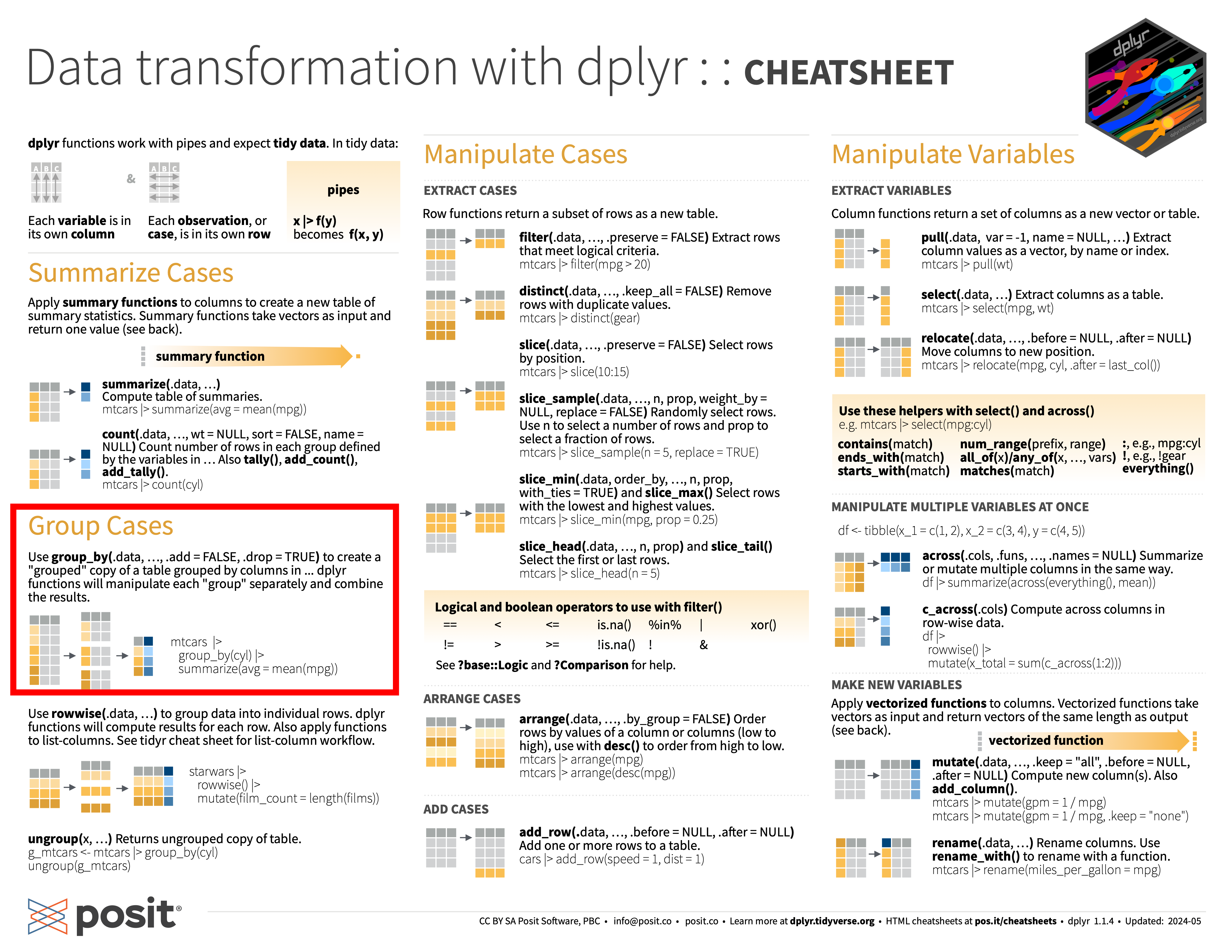
이상은 dplyr cheatsheet에서 다음 부분을 설명했다.
11.6 여러 열에 대한 오퍼레이션: across()을 중심으로
glimpse(penguins)Rows: 344
Columns: 8
$ species <fct> Adelie, Adelie, Adelie, Adelie, Adelie, Adelie, Adelie, Ad…
$ island <fct> Torgersen, Torgersen, Torgersen, Torgersen, Torgersen, Tor…
$ bill_len <dbl> 39.1, 39.5, 40.3, NA, 36.7, 39.3, 38.9, 39.2, 34.1, 42.0, …
$ bill_dep <dbl> 18.7, 17.4, 18.0, NA, 19.3, 20.6, 17.8, 19.6, 18.1, 20.2, …
$ flipper_len <int> 181, 186, 195, NA, 193, 190, 181, 195, 193, 190, 186, 180,…
$ body_mass <int> 3750, 3800, 3250, NA, 3450, 3650, 3625, 4675, 3475, 4250, …
$ sex <fct> male, female, female, NA, female, male, female, male, NA, …
$ year <int> 2007, 2007, 2007, 2007, 2007, 2007, 2007, 2007, 2007, 2007…across() 함수를 이해하고 잘 활용하려면 약간의 배경 지식이 필요하다. 먼저 함수형 프로그래밍(functional programming) 기법이다.
베이스 R에서 lapply(), sapply() 함수는 대표적인 함수형 프로그래밍 함수이다. 이 함수들은 데이터 프레임이나 리스트에 대하여 반복적으로 함수를 적용하여 결과를 반환한다. 예를 들어, 다음과 같은 데이터 프레임이 있다고 하자.
df <- data.frame(
    x = 1:3,
    y = 4:6,
    z = 7:9
)
이 데이터 프레임에 대하여 lapply() 함수를 적용하면 다음과 같은 결과를 얻을 수 있다. 두 번째 인자로 각 열에 대하여 적용할 함수(이름)을 전달한다는 점을 주의한다. 이처럼 함수를 하나의 값으로 사용하여 프로그래밍하는 기법을 함수형 프로그래밍이라고 한다.
lapply(df, mean)$x
[1] 2
$y
[1] 5
$z
[1] 8sapply() 함수는 이 결과를 벡터로 반환한다.
sapply(df, mean)x y z
2 5 8 lappy(), sapply() 함수의 두 번째 인자는 함수이다. 이 함수는 데이터 프레임의 각 열에 대하여 적용된다. 만약 우리가 원하는 것을 계산하는 함수가 없으면 직접 만들어서 사용할 수 있고, lapply(), sapply() 함수 안에서 바로 정의하여 사용할 수 있는데, 이런 경우 이름이 없는 함수인 익명 함수(anonymous function)를 사용한다.
R에서 익명 함수는 베이스 R과 특정 패키지를 이용하는 방법들이 존재했는데, R 4.1.0 버전부터는 네이티브로 지원한다. Tidyverse에서도 purrr 패키지를 통해서 R 포뮬러(~)을 이용한 익명 함수를 사용했었는데, 이제는 네이티브 익명함수를 사용하는 쪽으로 권장되고 있다.
R에서 익명 함수 만들기
버전 4.1.0 이전에서 베이스 R로 익명함수는 다음과 같이 만들었다.
lapply(df, function(x) mean(x, na.rm = TRUE))버전 4.1.0 이후에서는 네이티브로 지원하므로 다음과 같이 만들면 된다.
lapply(df, \(x) mean(x, na.rm = TRUE))
11.6.1 across() 함수
- 사용할 데이터
- palmerpenguins
- 2025년 4월 새로 업데이트된 R 4.5.0 버전에
palmerpenguins이 base R에 포함되었다.

다음과 같은 코드로 현재 사용하는 R 버전을 확인할 수 있다.
> R.version.string[1] "R version 4.5.1 (2025-06-13)"across() 함수는 주로 summarise() 함수와 함꼐 사용된다. 첫 번째 인자는 .cols로 함수를 적용시킬 열을 선택하고, 두 번째 인자는 .fns로 적용시킬 함수를 지정한다.
다음은 where(is.numeric) 함수를 사용하여 penguins 데이터셋에서 모든 숫자형 변수들에 대하여 평균을 계산하는 예이다.
  bill_len bill_dep flipper_len body_mass     year
1 43.92193 17.15117    200.9152  4201.754 2008.029
다음은 모든 행에서 unique한 값의 개수를 계산하는 예이다.
penguins |>
    summarise(across(
        everything(),
        n_distinct
    ))
species island bill_len bill_dep flipper_len body_mass sex year
1 3 3 165 81 56 95 3 3
11.6.2 여러 행에 대한 오퍼레이션: rowwise() 함수
rowwise() 함수는 각 행 단위로 함수를 적용시킬 때 사용한다.
# A tibble: 2 × 4
  name       x     y     z
  <chr>  <int> <int> <int>
1 Mara       1     3     5
2 Hadley     2     4     6
먼저 rowwise() 함수를 사용하지 않을 때를 생각해 보자. 다음 코드는 df 데이터프레임을 구성하는 x,y, z 열을 모두 더하는 방식으로 평균을 구한다.
# A tibble: 2 × 5
  name       x     y     z     m
  <chr>  <int> <int> <int> <dbl>
1 Mara       1     3     5   3.5
2 Hadley     2     4     6   3.5
만약 각 행에 대한 평균을 구하고자 한다면, rowwise() 함수를 사용하여 각 행에 대하여 평균을 계산한다.
# A tibble: 2 × 5
# Rowwise:
  name       x     y     z     m
  <chr>  <int> <int> <int> <dbl>
1 Mara       1     3     5     3
2 Hadley     2     4     6     4
이렇게 열이 몇 개 되지 않을 때는 문제가 없지만, 열이 많은 경우에는 c_across() 함수를 사용하면 select() 함수에서 열을 선택하는 방법을 적용시킬 수 있다.
# A tibble: 344 × 9
# Rowwise:
   species island    bill_len bill_dep flipper_len body_mass sex     year     m
   <fct>   <fct>        <dbl>    <dbl>       <int>     <int> <fct>  <int> <dbl>
 1 Adelie  Torgersen     39.1     18.7         181      3750 male    2007  997.
 2 Adelie  Torgersen     39.5     17.4         186      3800 female  2007 1011.
 3 Adelie  Torgersen     40.3     18           195      3250 female  2007  876.
 4 Adelie  Torgersen     NA       NA            NA        NA <NA>    2007  NaN
 5 Adelie  Torgersen     36.7     19.3         193      3450 female  2007  925.
 6 Adelie  Torgersen     39.3     20.6         190      3650 male    2007  975.
 7 Adelie  Torgersen     38.9     17.8         181      3625 female  2007  966.
 8 Adelie  Torgersen     39.2     19.6         195      4675 male    2007 1232.
 9 Adelie  Torgersen     34.1     18.1         193      3475 <NA>    2007  930.
10 Adelie  Torgersen     42       20.2         190      4250 <NA>    2007 1126.
# ℹ 334 more rows
11.7 테이블 대상 동사
이 내용을 이해하기 위해서는 관계형 데이터베이스에 관한 기본적인 이해가 선행되어야 하기 때문에 14장에서 따로 설명한다.