f <- y ~ x + b
class(f)
[1] "formula"R 언어에서는 통계적 모델(statistical model)을 표현하기 위해 포뮬러(formula)를 사용한다. R 언어의 관점에서는 이것 역시 벡터나 데이터프레임, 리스트와 같은 객체의 한 종류이다.
포뮬러는 모델의 독립변수와 종속변수 간의 관계를 나타내는 상징적인 수식이다. 여기서 상징적 수식이라고 하는 것은 보통의 수학적 표현이 아니라는 뜻이다. R 언어에서 특별한 역할을 하는 표현식의 일종이다.
R에서 많은 통계 분석 함수나 그래픽 함수들이 이 포뮬러를 사용하기 때문에 잘 이해할 필요가 있고, 실제로도 많은 데이터 분석 작업에서 포뮬러를 사용한다.
f <- y ~ x + b
class(f)[1] "formula"~ 기호를 중심으로 왼쪽은 종속 변수(dependent variable), 오른쪽은 독립 변수(independent variable)를 표시한다. 대부분 이런 변수들은 데이터프레임의 열 이름을 사용한다. 이 f라는 객체는 formula 클래스의 객체이다.
포뮬러를 정의할 때는 표 27.1에 있는 기호들을 사용한다.
| 기호 | 역할 | 예시 | 통계적의미 |
|---|---|---|---|
| ~ | 포뮬러의 좌변과 우변을 구분 | y ~ x | regress y on x |
| + | 포뮬러에 변수 추가함 | y ~ x + z | regress y on x and z |
| . | 모든 변수를 사용 | y ~ . | regress y on all other variables in a data frame |
| - | 포뮬러에서 변수를 뺌 | y ~ . - x | regress y on all other variables except x |
| 1 | Y 절편 포함 | y ~ x - 1 | regress y on x without an intercept |
| : | 상호작용 | y ~ x + z + x:z | regress y on x, z, and the product x times z |
| * | factor crossing | y ~ x * z | regress y on x, z, and the product x times z |
| ^ | 고차원 상호작용 | y ~ (x + z + w)^3 | regress y on x, z, w, all two-way interactions, and the three-way interactions |
| I() | 안에 수식을 진짜 수식으로 사용 | y ~ x + I(x^2) | regress y on x and x squared |
* 기호는 factor crossing을 의미한다. a*b는 a + b + a:b와 같다.
^ 기호는 고차원 상호작용을 의미한다. (a+b+c)^2는 a + b + c + a:b + a:c + b:c와 같다.
I() 기호는 안에 있는 것이 진짜 수식으로 사용된다는 것을 의미한다.
다음 자료는 Tidymodeling with R 책에서 인용하였다.
귀뛰라미(crickets) 데이터는 온도와 귀뛰라미의 초당 소리 횟수 간의 관계를 나타내는 데이터이고, 2개의 아종별에 대해 조사했다.
[1] "species" "temp" "rate" # Plot the temperature on the x-axis, the chirp rate on the y-axis. The plot
# elements will be colored differently for each species:
ggplot(
crickets,
aes(x = temp, y = rate, color = species, pch = species, lty = species)
) +
# Plot points for each data point and color by species
geom_point(size = 2) +
# Show a simple linear model fit created separately for each species:
geom_smooth(method = lm, se = FALSE, alpha = 0.5) +
scale_color_brewer(palette = "Paired") +
labs(x = "Temperature (C)", y = "Chirp Rate (per minute)")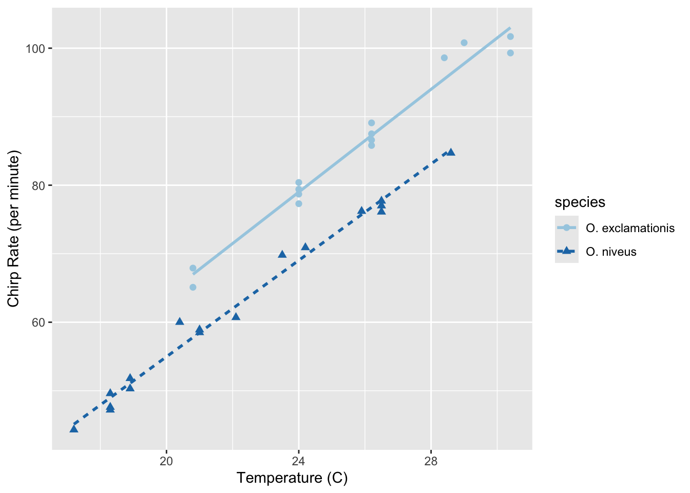
위 그래프를 보면 온도와 귀뛰라미의 초당 소리 횟수 간의 선형 관계가 있고, 각 아종이 서로 다르다는 것을 볼 수 있다.
먼저 lm() 함수를 사용하는데, 이 함수는 R 포뮬러와 데이터프레임을 인자로 받는다. 먼저 소리 횟수와 온도와 관계를 R 포뮬러로 다음과 같이 표현할 수 있다.
rate ~ temp종속 변수 rate가 독립 변수 temp에 의해 설명된다는 것을 의미한다.
만약 아종에 대한 변수를 독립 변수로 추가하려면 다음과 같은 포뮬러를 사용할 수 있다.
rate ~ temp + species이 경우 species는 범주형 변수이다. 이 포뮬러는 온도와 아종에 대한 영향을 동시에 고려한다는 것을 의미한다. 이런 범주형 변수는 모델 fitting 과정에서 숫자형으로 변환된 다음 계산된다.
temp와 species이 상호작용(interaction)을 하는 경우 다음과 같은 포뮬러를 사용할 수 있다. 변수들간의 상호작용은 콜론(:)으로 표현한다.
rate ~ temp + species + temp:species위 포뮬러는 다음과 같은 단축형으로도 표현할 수 있는데, 모두 같은 의미이다.
rate ~ temp * species
rate ~ (temp + species)^2
이제 모델 fitting을 해보자.
interaction_fit <- lm(rate ~ (temp + species)^2, data = crickets)이렇게 해서 만들어진 interaction_fit 객체는 여러 정보를 담고 있다.
interaction_fit
Call:
lm(formula = rate ~ (temp + species)^2, data = crickets)

Coefficients:
          (Intercept)                   temp       speciesO. niveus
              -11.041                  3.751                 -4.348
temp:speciesO. niveus
-0.234 summary(interaction_fit)
Call:
lm(formula = rate ~ (temp + species)^2, data = crickets)

Residuals:
    Min      1Q  Median      3Q     Max
-3.7031 -1.3417 -0.1235  0.8100  3.6330

Coefficients:
                      Estimate Std. Error t value Pr(>|t|)
(Intercept)           -11.0408     4.1515  -2.659    0.013 *
temp                    3.7514     0.1601  23.429   <2e-16 ***
speciesO. niveus       -4.3484     4.9617  -0.876    0.389
temp:speciesO. niveus  -0.2340     0.2009  -1.165    0.254
---
Signif. codes:  0 '***' 0.001 '**' 0.01 '*' 0.05 '.' 0.1 ' ' 1

Residual standard error: 1.775 on 27 degrees of freedom
Multiple R-squared:  0.9901,    Adjusted R-squared:  0.989
F-statistic: 898.9 on 3 and 27 DF,  p-value: < 2.2e-16
이제 모델을 시각화해보자.
# Place two plots next to one another:
par(mfrow = c(1, 2))

# Show residuals versus predicted values:
plot(interaction_fit, which = 1)

# A normal quantile plot on the residuals:
plot(interaction_fit, which = 2)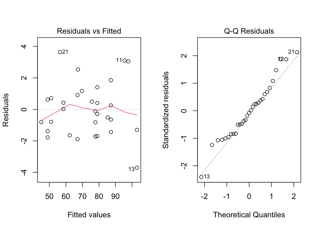
인터랙션 term이 필요한지를 확인하기 위해 인터랙션 term이 없는 모델을 보자.
main_effects_fit <- lm(rate ~ temp + species, data = crickets)인터랙션이 있는 모델과 없는 모델의 차이를 anova() 함수를 사용하여 비교할 수 있다.
anova(main_effects_fit, interaction_fit)Analysis of Variance Table
Model 1: rate ~ temp + species
Model 2: rate ~ (temp + species)^2
Res.Df RSS Df Sum of Sq F Pr(>F)
1 28 89.350
2 27 85.074 1 4.2758 1.357 0.2542P-값이 0.25로 인터랙션 term이 필요하지 않다는 귀무 가설을 기각할 수 없다.
summary(main_effects_fit)
Call:
lm(formula = rate ~ temp + species, data = crickets)

Residuals:
    Min      1Q  Median      3Q     Max
-3.0128 -1.1296 -0.3912  0.9650  3.7800

Coefficients:
                  Estimate Std. Error t value Pr(>|t|)
(Intercept)       -7.21091    2.55094  -2.827  0.00858 **
temp               3.60275    0.09729  37.032  < 2e-16 ***
speciesO. niveus -10.06529    0.73526 -13.689 6.27e-14 ***
---
Signif. codes:  0 '***' 0.001 '**' 0.01 '*' 0.05 '.' 0.1 ' ' 1

Residual standard error: 1.786 on 28 degrees of freedom
Multiple R-squared:  0.9896,    Adjusted R-squared:  0.9888
F-statistic:  1331 on 2 and 28 DF,  p-value: < 2.2e-16
이렇게 만들어진 모델을 사용하여 예측(prediction)을 할 수 있다.
new_values <- data.frame(species = "O. exclamationis", temp = 15:20)
predict(main_effects_fit, new_values)
1 2 3 4 5 6
46.83039 50.43314 54.03589 57.63865 61.24140 64.84415