library(ggplot2)
library(gghighlight)
library(tidyverse)

ggplot(data.frame(x = c(-4, 4)), aes(x)) +
    stat_function(fun = dnorm, args = list(mean = 0, sd = 1)) +
    theme_minimal()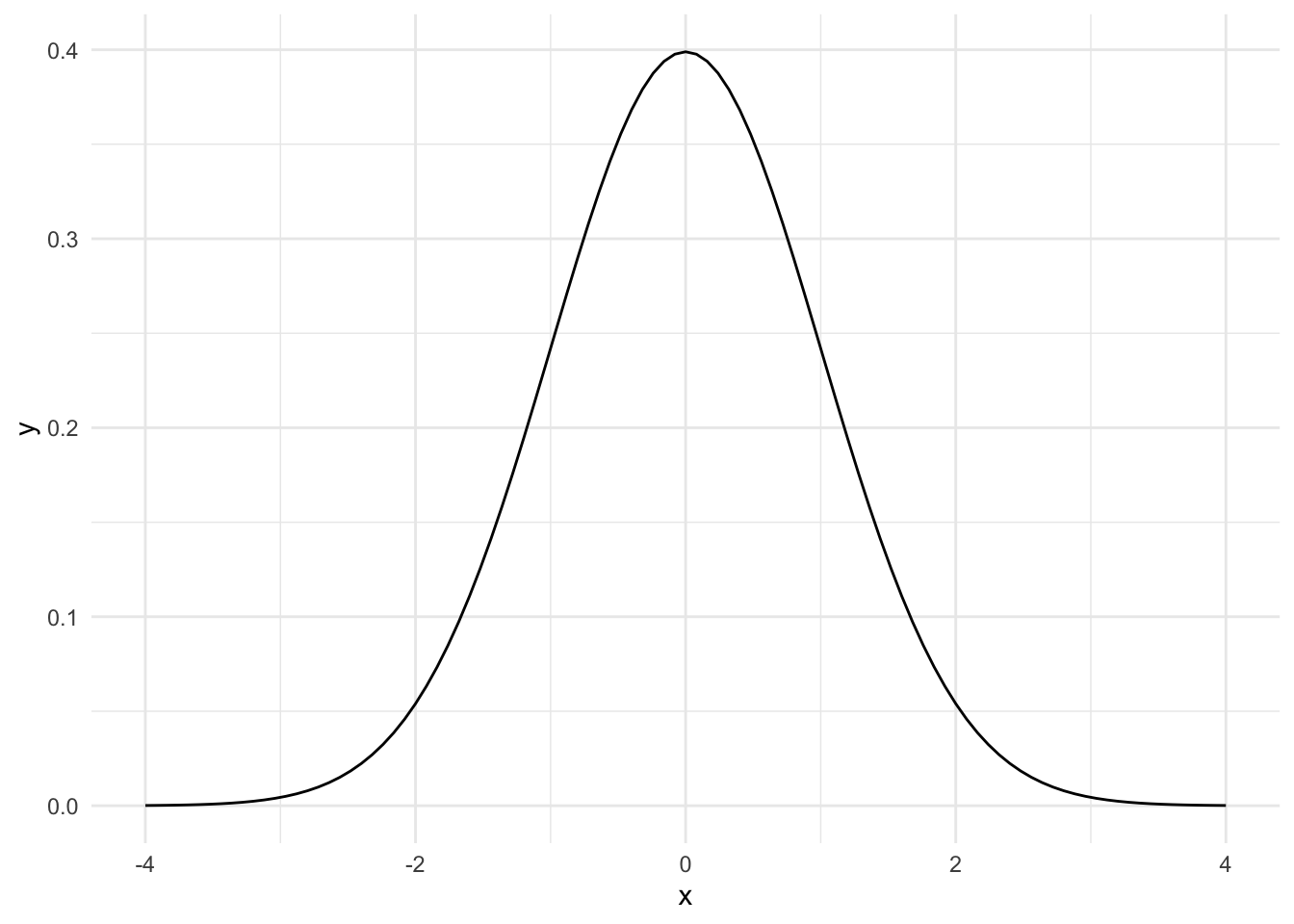
tidymodels 패키지에 포함된 infer 패키지는 가설 검정(hypothesis testing)을 위한 표준적이고 일반적인 프레임워크를 제공한다. 개별 통계 함수나 특정 패키지를 사용하는 것보다는 좀 더 일반적이고 일관된 접근법을 취할 수 있고, 무엇보다 가설 검정의 의미를 이해하면서 가설 검정을 할 수 있다는 장점을 가지고 있다.
가설 검정의 일반적인 방법은 다음과 같다.
여기서 통계량(statistic)은 데이터의 특정 특성을 수치로 나타낸 것을 의미한다. 예를 들어, 평균, 비(proportion), 중앙값, 표준편차, 상관계수 등이 통계량에 해당한다.
귀무 가설(null hypothesis)은 “아무런 차이가 없다”는 것을 의미한다. 예를 들어, 두 그룹의 평균이 같다고 가정하는 것을 말한다.
귀무 분포(null distribution)는 귀무 가설을 바탕으로 생성된 확률 분포(probability distribution)를 의미한다.
R에는 알려진 분포들에 대한 여러 함수들을 제공하고, 다음과 같은 접두사를 사용한다. 베이스 R에서 제공되는 분포는 ?distributions를 참고하자. 정규분포(norm1), t 분포(t), F 분포(f) 등 다양하게 준비되어 있다.
d: 확률 밀도(density) 함수, 확률 밀도 함수는 확률 변수가 특정 값을 가질 확률을 나타내는 함수이다.p: 누적 분포(cumulative distribution) 함수, 누적 분포 함수는 확률 변수가 특정 값 이하일 확률을 나타내는 함수이다.q: 분위수(quantile) 함수, 분위수 함수는 확률 변수가 특정 값 이하일 확률이 특정 값일 때, 그 값을 찾는 함수이다.r: 랜덤 샘플(random sample) 생성 함수, 랜덤 샘플 생성 함수는 확률 변수가 특정 분포를 따를 때, 그 분포에서 랜덤하게 샘플을 생성하는 함수이다.
확률 변수 x가 표준정규분포를 따른다고 해 보자. 이 x는 우리가 구하려고 하는 어떤 통계량이라고 생각하자.
평균이 0이고 표준편차가 1인 정규분포를 ggplot2 패키지를 사용해 시각화해 보자.
library(ggplot2)
library(gghighlight)
library(tidyverse)
ggplot(data.frame(x = c(-4, 4)), aes(x)) +
stat_function(fun = dnorm, args = list(mean = 0, sd = 1)) +
theme_minimal()
x <= 2일 때의 확률은 다음과 같이 계산할 수 있다.
pnorm(2, mean = 0, sd = 1)[1] 0.9772499이것을 시각화해 보자.
ggplot(data = tibble(x = -4:4), mapping = aes(x = x)) +
    stat_function(fun = dnorm) +
    stat_function(
        fun = function(x) ifelse(x < 2, dnorm(x), NA),
        geom = "area",
        fill = "sky blue"
    ) +
    theme_minimal()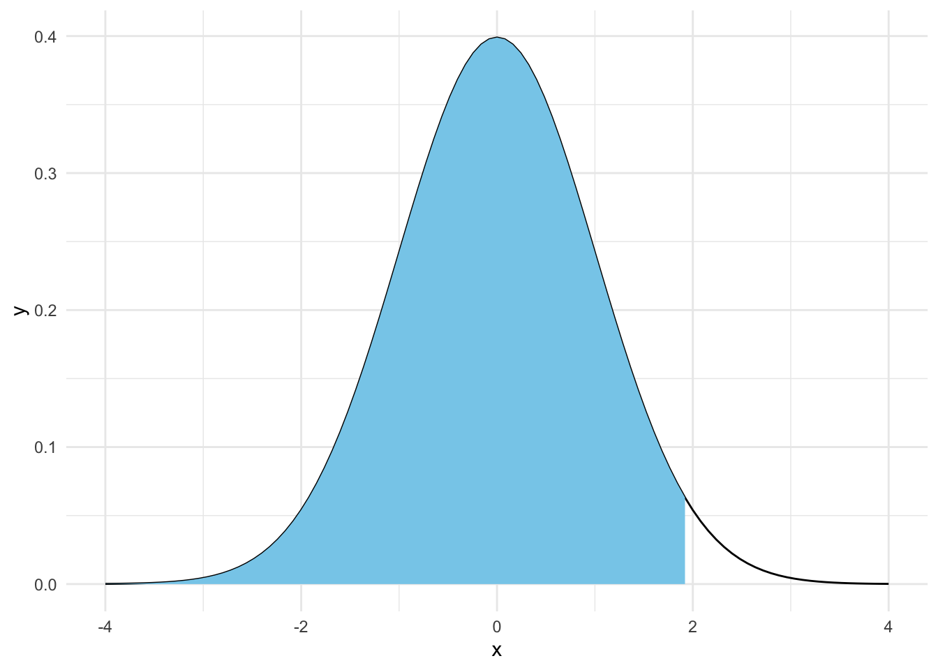
x >= 2일 때의 확률은 다음과 같이 계산할 수 있다. 이것이 p-value와 관련되어 있다.
1 - pnorm(2, mean = 0, sd = 1)[1] 0.02275013이것을 시각화해 보자.
ggplot(data = tibble(x = -4:4), mapping = aes(x = x)) +
    stat_function(fun = dnorm) +
    stat_function(
        fun = function(x) ifelse(x > 2, dnorm(x), NA),
        geom = "area",
        fill = "sky blue"
    ) +
    theme_minimal()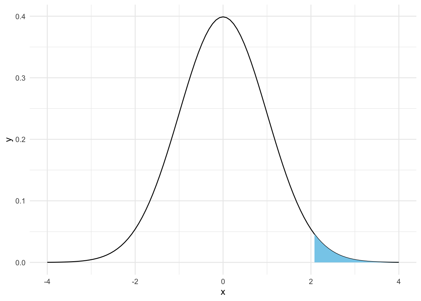
infer 패키지에서는
X = 2와 같이 관찰된 통계량이 귀무 분포에서 나올 확률을 계산한다.p-value이다.infer 패키지의 기본 개념infer 패키지는 모델 추정 및 모델 검정을 위한 패키지로, 4개의 핵심 동사(함수)를 기반으로 가설 검정에 대한 일반적인 프레임워크를 제공한다. 이 4개 핵심 동사를 통해 모델을 설정하고, 귀무 가설을 설정하고, 귀무 분포를 생성하고, 통계량을 계산한다.
specify() : 변수들의 관계를 통해 모델을 설정hypothesize() : 귀무 가설을 설정generate() : 귀무 가설을 바탕으로 (샘플링 또는 이론에 근거하여) 귀무 분포를 생성calculate() : 관찰된 현재의 데이터를 바탕으로 통계량을 계산함.이들 동사와 더불어 다음과 같은 보조 함수를 사용한다.
visualize() : 분포 시각화
shade_p_value() : p-value 영역 시각화shade_confidence_interval() : 신뢰 구간 시각화get_p_value() : p-value 계산get_confidence_interval() : 신뢰 구간 계산이것은 ModernDive 책에서 언급하는 바와 같이 Aleln Downey의 가설 검정 프레임워크와 맥을 같이 한다.
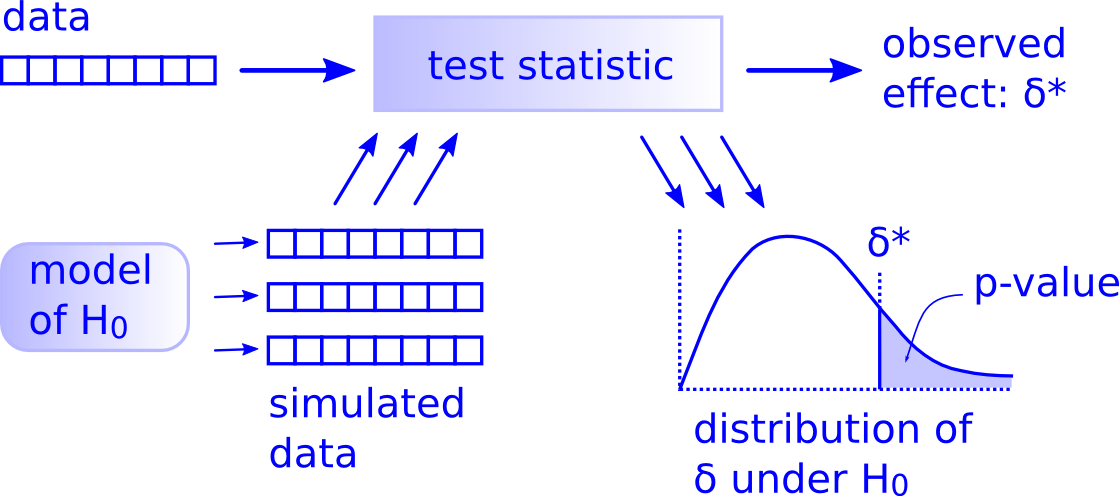
실제로 infer 패키지를 사용하려면 이런 프레임워크를 이해한 다음, 여러 상황에 따라 어떤 옵션이나 조건을 사용할지 결정하게 된다.
gss 데이터셋infer 패키지에는 미국에서 시행된 설문 데이터인 gss 데이터셋이 포함되어 있다. 이 데이터셋을 사용하여 infer 패키지 사용법을 익히자. 변수의 의미는 ?gss를 참고하자.
Rows: 500
Columns: 11
$ year    <dbl> 2014, 1994, 1998, 1996, 1994, 1996, 1990, 2016, 2000, 1998, 20…
$ age     <dbl> 36, 34, 24, 42, 31, 32, 48, 36, 30, 33, 21, 30, 38, 49, 25, 56…
$ sex     <fct> male, female, male, male, male, female, female, female, female…
$ college <fct> degree, no degree, degree, no degree, degree, no degree, no de…
$ partyid <fct> ind, rep, ind, ind, rep, rep, dem, ind, rep, dem, dem, ind, de…
$ hompop  <dbl> 3, 4, 1, 4, 2, 4, 2, 1, 5, 2, 4, 3, 4, 4, 2, 2, 3, 2, 1, 2, 5,…
$ hours   <dbl> 50, 31, 40, 40, 40, 53, 32, 20, 40, 40, 23, 52, 38, 72, 48, 40…
$ income  <ord> $25000 or more, $20000 - 24999, $25000 or more, $25000 or more…
$ class   <fct> middle class, working class, working class, working class, mid…
$ finrela <fct> below average, below average, below average, above average, ab…
$ weight <dbl> 0.8960034, 1.0825000, 0.5501000, 1.0864000, 1.0825000, 1.08640…hours)Response: hours (numeric)
# A tibble: 1 × 1
stat
<dbl>
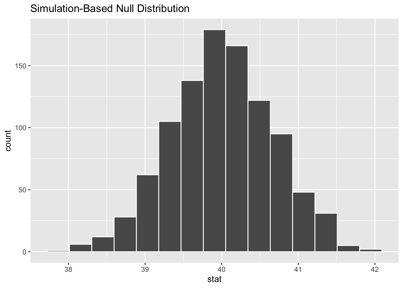
1 41.4귀무 가설을 바탕으로 귀무 분포를 생성한다. bootstrap 방법을 사용하여 귀무 분포를 생성한다.
위 코드의 의미는 다음과 같다.
specify(response = hours): 지난 주 근무한 시간을 응답 변수로 지정한다.hypothesize(null = "point", mu = 40): 귀무 가설을 설정한다. 귀무 가설은 평균이 40이다. 구간이 아닌 포인트 가설이다.generate(reps = 1000, type = "bootstrap"): 귀무 가설을 바탕으로 귀무 분포를 생성한다. bootstrap 방법을 사용하여 귀무 분포를 생성한다. 1000번 반복하여 샘플을 확보한다.calculate(stat = "mean"): 샘플에 대한 평균을 구한다.귀무 분포를 시각화해 보자. visualize() 함수는 귀무 분포를 시각화한다.
이제 앞에서 관찰된 평균이 이 분포에 어떻게 위치하는지 확인해 보자.
null_dist_hours %>%
visualize() +
shade_p_value(obs_mean_hours, direction = "two-sided")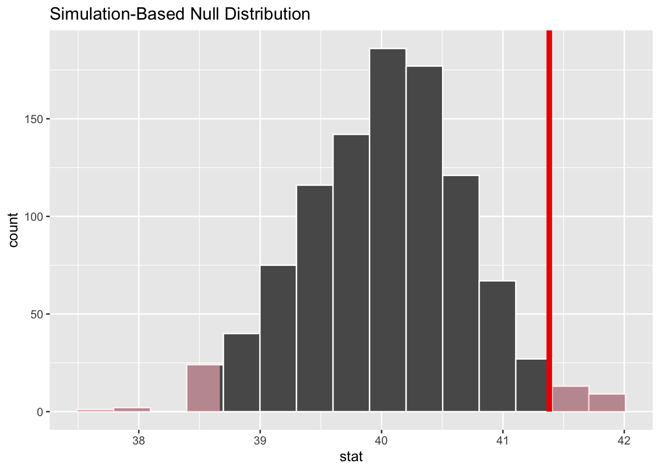
이제 이 분포에서 관찰된 평균이 나올 확률을 계산해 보자.
null_dist_hours %>%
    get_p_value(obs_mean_hours, direction = "two-sided")
# A tibble: 1 × 1
p_value
<dbl>
1 0.048t_test(gss, response = hours, mu = 40)# A tibble: 1 × 7
statistic t_df p_value alternative estimate lower_ci upper_ci
<dbl> <dbl> <dbl> <chr> <dbl> <dbl> <dbl>
1 2.09 499 0.0376 two.sided 41.4 40.1 42.7# calculate the observed statistic
observed_statistic <- gss %>%
specify(response = hours) %>%
hypothesize(null = "point", mu = 40) %>%
calculate(stat = "t") %>%
dplyr::pull()
observed_statistic t
2.085191 library(dplyr)
library(knitr)
library(readr)
ageAtMar <- read_csv("https://ismayc.github.io/teaching/sample_problems/ageAtMar.csv")Rows: 5534 Columns: 1
── Column specification ────────────────────────────────────────────────────────
Delimiter: ","
dbl (1): age
ℹ Use `spec()` to retrieve the full column specification for this data.
ℹ Specify the column types or set `show_col_types = FALSE` to quiet this message.glimpse(ageAtMar)Rows: 5,534
Columns: 1
$ age <dbl> 32, 25, 24, 26, 32, 29, 23, 23, 29, 27, 23, 21, 29, 40, 22, 20, 31…ageAtMar %>% ggplot(aes(x = age)) +
geom_histogram(binwidth = 3, color = "white")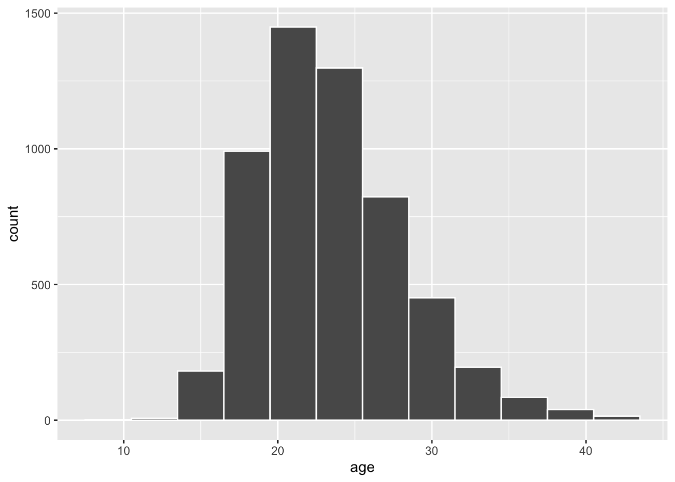
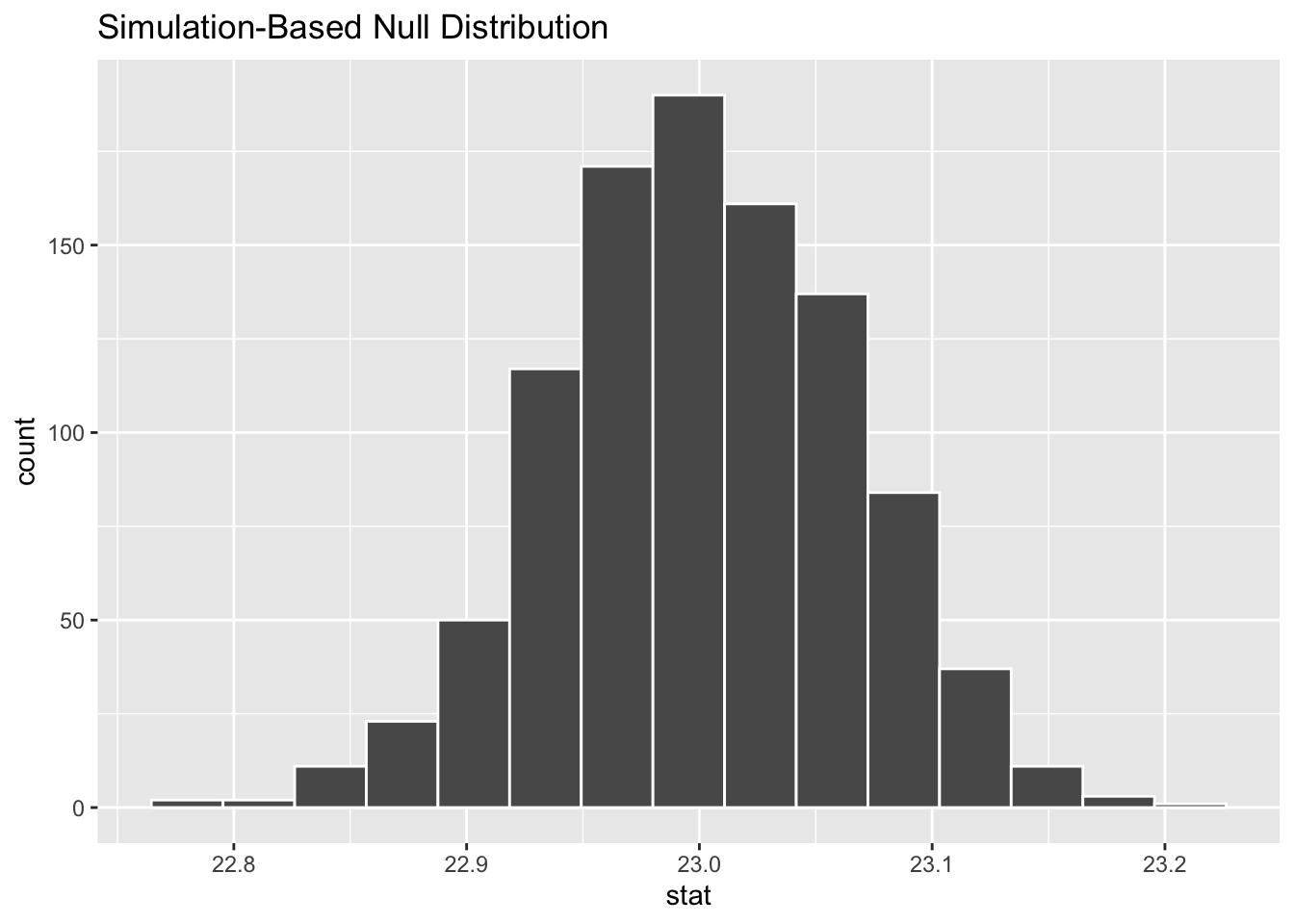
관찰된 나이의 평균은 다음과 같다.
Response: age (numeric)
# A tibble: 1 × 1
   stat
  <dbl>
1  23.4
귀무 가설을 바탕으로 귀무 분포를 생성한다. bootstrap 방법을 사용하여 귀무 분포를 생성한다.
귀무 분포를 시각화해 보자.
이제 앞에서 관찰된 평균이 이 분포에 어떻게 위치하는지 확인해 보자.
null_dist_age %>%
visualize() +
shade_p_value(obs_mean_age, direction = "two-sided")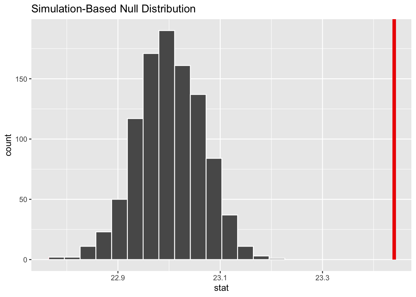
이제 이 분포에서 관찰된 평균이 나올 확률을 계산해 보자.
null_dist_age %>%
    get_p_value(obs_mean_age, direction = "two-sided")
Warning: Please be cautious in reporting a p-value of 0. This result is an approximation
based on the number of `reps` chosen in the `generate()` step.
ℹ See `get_p_value()` (`?infer::get_p_value()`) for more information.# A tibble: 1 × 1
p_value
<dbl>
1 0신뢰 구간을 계산해 보자.
null_dist_age %>%
    get_confidence_interval(level = 0.95)
# A tibble: 1 × 2
lower_ci upper_ci
<dbl> <dbl>
1 22.9 23.1t_test()를 시행해 보자.
t_test(ageAtMar, response = age, mu = 23)# A tibble: 1 × 7
statistic t_df p_value alternative estimate lower_ci upper_ci
<dbl> <dbl> <dbl> <chr> <dbl> <dbl> <dbl>
1 6.94 5533 4.50e-12 two.sided 23.4 23.3 23.6# calculate the observed statistic
observed_statistic <- ageAtMar %>%
specify(response = age) %>%
hypothesize(null = "point", mu = 23) %>%
calculate(stat = "t") %>%
dplyr::pull()
observed_statistic t
6.935697